Predict Movie Sentiment via DOC2VEC

In order to have an introduction of the Word2Vec look at this post. Using this method we try to predict the movie sentiment (positive vs. negative) using text data as predictor. We use the movie review data set, and we use the power of Doc2Vec to transform our data into predictors.

library(text2vec)
library(tm)

data(movie_review)
names(movie_review)

[1] "id"        "sentiment" "review"   

The data set contain an id, sentiment (0=negative, 1=positive), and review that contains the text if people like the movie or not. We start creating the Training and Test set, and we have also to collect unique terms from the document using the function create_vocabulary().

library(caret)
Train = createDataPartition(movie_review$sentiment, p=0.75, list=FALSE, times = 1) # function to devide training and test set

# Define training control
# train_control =trainControl(method="cv", number=10)
train = movie_review[Train, ] # 75% training
test = movie_review[-Train, ] # 25% test

# TRAINING-SET
# Vocabulary-based DTM
# We collect unique terms from all documents and mark each of them with a unique ID using the create_vocabulary() function
it = itoken(train$review, preprocessor = tolower, # transform text to lowercase
            tokenizer = word_tokenizer,           # create a token
            ids = train$id)                       # assign id


# Iterator over tokens with the itoken() function
v = create_vocabulary(it)

# Represent documents in vector space
vectorizer = vocab_vectorizer(v)




# TEST-SET
it2 = itoken(test$review, preprocessor = tolower,
             tokenizer = word_tokenizer,
             ids = test$id)
# v2 = create_vocabulary(it2)
# pruned_vocab2 = prune_vocabulary(v2, term_count_min = 10, doc_proportion_max = 0.5, doc_proportion_min = 0.001)
# vectorizer2 = vocab_vectorizer(v2)

# Document term matrix (vocab based)
dtm_train = create_dtm(it, vectorizer) # training set
dtm_test = create_dtm(it2, vectorizer) # test set

Now, we have to get the tf-idf matrix from the bag of words.
The bag of words is used to extract features. We simply count the number of occurrences for each word, this process in also called CountVectorizer.
To make the CountVectorizer more comparable, we scale it using the Term Frequency Transformation (tf) and in order to boost the most important features we use the Inverse Document Frequency (IDF), this calculate how often a word occurs in the corpus. The combination of both is called tf-idf = tf * idf. The tf-idf can be also represented as follow:

\[ i d f(t, D)=\log \left(\frac{N}{|\{d \in D : t \in d\}|}\right) \] The tf-idf is the log of the total number of documents N divided by the number of documents that contain the term that we are taking into consideration.

# Get tf-idf 
# It quantify importance of a term in a document
# Increase the weight of terms which are specific to a single document decrease the weight for terms used in most documents

tfidf <- TfIdf$new() # define tfidf model

# Implement the tfidf model to the training and test set
dtm_train_tfidf <- fit_transform(dtm_train, tfidf)
dtm_test_tfidf <- fit_transform(dtm_test, tfidf)

Now, we are ready to use the Sparse Linear Model with the R package glmnet that works quite well when we have to deal with binary response variable. In Document Classification we might have a lange number of variables per observation. We cannot fit the data using standard approaches since p>>N, where p=features and N=document samples.
The Sparse Linear Model tries to optimize each parameter separately holding all the other parameters fixed, and it does it on a grid of lambda. For an exhaustive explanation of Sparse Linear Model there is a great lesson that you can find here.

# GLMNET model
library(glmnet)

glmnet_classifier =cv.glmnet(x = dtm_train_tfidf, y = train[['sentiment']], # predict sentiment
                             family = 'binomial',  # because we are dealing with a binary responce variable
                             alpha = 1,            # L1 penalty
                             type.measure = "auc", # area under ROC curve
                             nfolds = 5,           # 5-fold cross-validation
                             thresh = 1e-3,        # convergence threshold for coordinate descent, high value is less accurate, but has faster training
                             maxit = 1e3)          # limit the maximum number of variables in the model, we use lower number of iterations for faster training

plot(glmnet_classifier)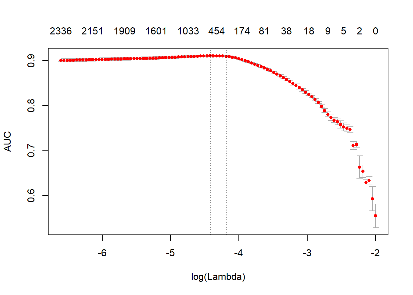

print(paste("max AUC =", round(max(glmnet_classifier$cvm), 4)))

[1] "max AUC = 0.9108"

# Predict on unseen data
preds <- predict(glmnet_classifier, dtm_test_tfidf, type= 'response')[, 1]
glmnet:::auc(as.numeric(test$sentiment), preds)

[1] 0.8922888

# How accurately can the sentiments be identified from text

As we can see from the graph above, we can determine the best value of lambda in order to have the best AUC. We also obtained a very high AUC aroud 90% in the Train Set, which is comparable to the Testing Set AUC 91%. This says to use that the model we created can predict the reviews of the unseen movie with a high level of Accuracy.