Time Series Clustering

Clustering is the task of grouping s set of objects in such a way that objects in the same group are more similar to each other than to those in other groups. Connectivity-based clustering connects objects to form clusters based on their distance. A cluster can be descibed by the maximum distance needed to connect parts of the cluster. At different distances, different clusters will form, which can be represented using dendrogram.

Time series clustering problems arise when we observe a sample of time series and we want to group them into different categories or clusters. This is a central problem in many application fields and hence time series clustering is nowadays an active research area in different disciplines including finance and economics, medicine, engineering, seismology and meteorology, among others.

We use the Synthetic Control Chart Time Series. This dataset contains 600 examples of control charts synthetically generated by the process in Alcock and Manolopoulos (1999).

data <- read.table("C:/07 - R Website/dataset/TS/synthetic_control.txt", header = FALSE)

plot(data[,60], type='l')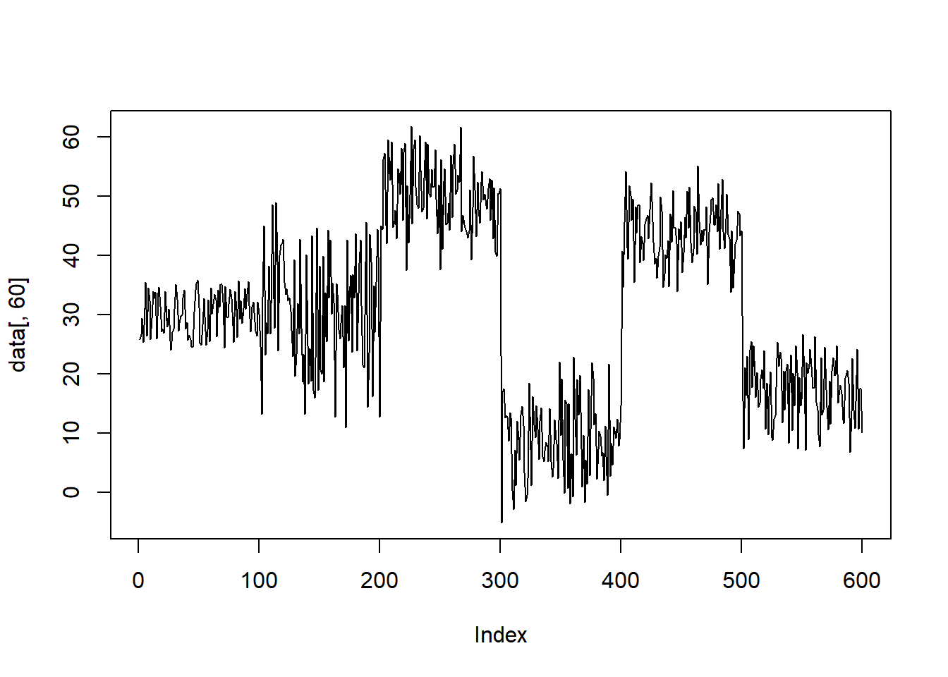

From the graph above, we can see the our data have six patterns. Now we try to separate ech of these six patterns.

# Separate the patterns
j <- c(5, 105, 205, 305, 405, 505)
sample <- t(data[j,])
plot.ts(sample)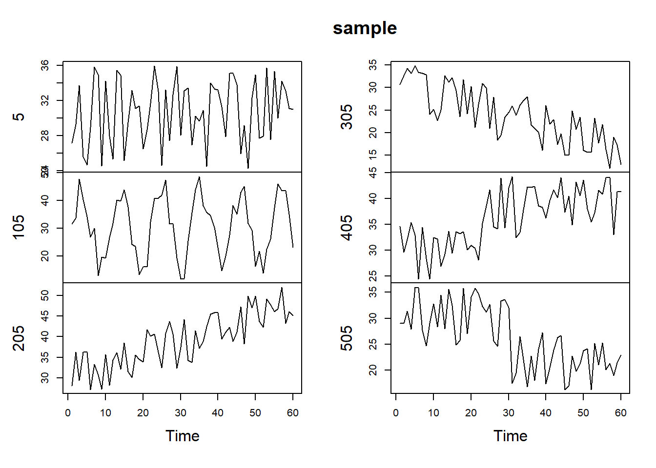

Starting from the top left graph, we have normal trend (5), cycle (105), increasing trend (205), decreasing trend (305), upward shift (405), downward shift (505). Now, we need to do same data preparationg before starting time series clustering.

# Data Preparation
n <- 10
s <- sample(1:100, n)
i <- c(s, 100+s,200+s, 300+s, 400+s, 500+s) # systematic random sample
d <- data[i,]

pattern <- c(rep('Normal', n),
             rep('Cyclic', n),
             rep('Increasing trend', n),
             rep('Decreasing trend', n),
             rep('Upward shift', n),
             rep('Downward shift', n))

# Calculate distance with Dynamic Time Warping
library(dtw)
distance <- dist(d, method="DTW")

# Hierarchical Clustering
hc <- hclust(distance, method='average')
plot(hc, 
     labels = pattern,
     cex = 0.7,
     hang = -1)

rect.hclust(hc, k=4)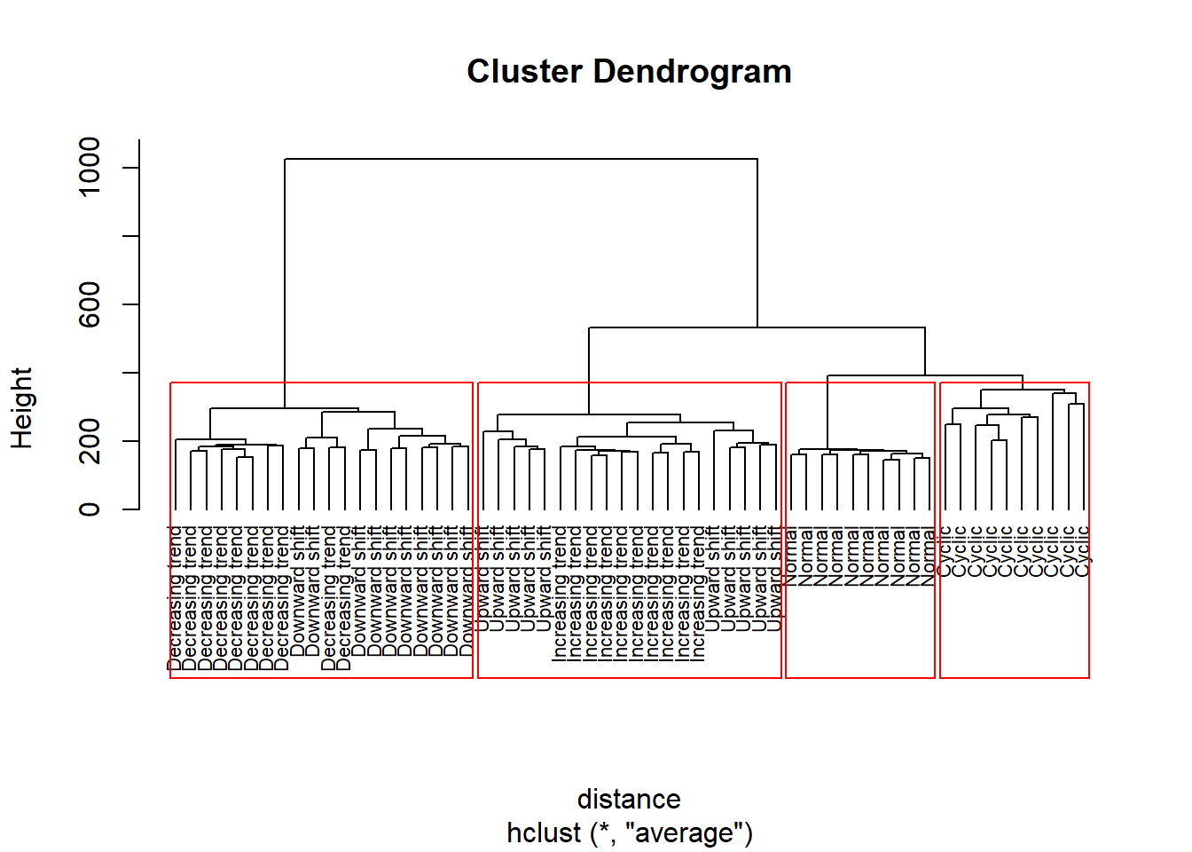

As we can see from the graph above, we calculated the distance using the Dynamic Time Warping. As we can see from the Cluster Dendrogram above, we have a well defined cluster for the Cyclic Time Series, and Normal Time Series. On the contrary, there is some mix between Downward shift Time Serie and Decreasing trend Time Serie, the same is between Upward shift Time Serie and Increasing trend Time Serie. This result in four clusters. but we already now that we have six clusters, in fact there is a problem to discriminate between Downward shift vs. Decreasing trend and Upward shift vs. Increasing trend.