In this post we will review the statistical background for time series analysis and forecasting. We start about how to compare different time seris models against each other.
Forecast Accuracy It determine how much difference thare is between the actual value and the forecast for the value. The simplest way to m ake a comparison is via scale dependent error because all the models need to be on the same scale using the Mean Absolute Error - MAE and the Root Mean Squared Error - RMSE. MAE is the mean of all differences between actual and forecaset absolute value and in order to avoid negative values we can use RMSE. We have also the Mean Absolute Scaled Error - MASE that measure the forecast error compared to the error of a naive forecast. When he have a MASE = 1, that means the model is exactly as good as just picking the last observation. An MASE = 0.5, means that our model has doubled the prediction accuracy. The lower, the better. When MASE > 1, that means the model needs a lot of improvement.
The Mean Absolute Percentage Error - MAPE, measures the difference of forecast errors and divides it by the actual observation value. The crucial point is that MAPE puts much more weight on extreme values and positive errors, which makes MASE a favor metrics. But the big benefit of MAPE is the fact that it is scale independent: that means we can use MAPe to compare a model on different datasets.
Quire often, Akaike Information Criterion - AIC is used. It is extensively used also in statistical modeling and machine learning to compare different models. The key point of AIC is that it penalizes more complex models.
We start as an example with a random time series. We divide the series into a training and a test set using the window() function. With window() function we can easily extract a time frame, in this case we take the part of the data starting from 1818 and ending in 1988. It is a beautiful fuction to split time series. The training data is used to fit the model and the test set is used to see how well the model performs.
set.seed(95)
myts <- ts(rnorm(200), start = (1818))
mytstrain <- window(myts, start = 1818, end = 1988) # training set
plot(mytstrain)

library(forecast)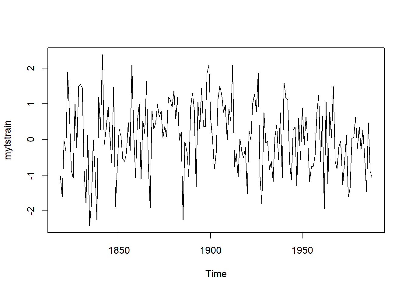
meanm <- meanf(mytstrain, h=30) # mean method and we get 30 observation in to the future
naivem <- naive(mytstrain, h=30) # naive method
drifm <- rwf(mytstrain, h=30, drift = TRUE) # drift method

mytstest <- window(myts, start = 1988)
accuracy(meanm, mytstest)
ME RMSE MAE MPE MAPE MASE
Training set 1.407307e-17 1.003956 0.8164571 77.65393 133.4892 0.7702074
Test set -2.459828e-01 1.138760 0.9627571 100.70356 102.7884 0.9082199
ACF1 Theil's U
Training set 0.1293488 NA
Test set 0.2415939 0.981051accuracy(naivem, mytstest) ME RMSE MAE MPE MAPE MASE
Training set -0.0002083116 1.323311 1.060048 -152.73569 730.9655 1.000000
Test set 0.8731935861 1.413766 1.162537 86.29346 307.9891 1.096683
ACF1 Theil's U
Training set -0.4953144 NA
Test set 0.2415939 2.031079accuracy(drifm, mytstest) ME RMSE MAE MPE MAPE MASE
Training set -8.988602e-15 1.323311 1.060041 -152.64988 730.8626 0.9999931
Test set 8.763183e-01 1.415768 1.163981 85.96496 308.7329 1.0980447
ACF1 Theil's U
Training set -0.4953144 NA
Test set 0.2418493 2.03317In the results we can see the error of both training and test set. It is also calculated the difference between the actual values from mytstest and the forecasted values from the model. As expected in all four of our statistics the mean method is the best, with the lowest value for RMSE, MAE, MAPE and MASE. That is as expected because we are working with a random data with zero mean and without any drift season.
The importance of Residuals in Time Series Analysis Residuals tell a lot about the quality of the model. The rule of thumb is: only randomness should stay in the residuals. They are the container of randomness (data that we cannot explain in mathematical terms) and ideally the have a mean of zero and constant variance. Residuals should be uncorrelated, correlated residuals still have information left in them, and ideally they are normally distributed. That is aso caed random walk (each vaue is a random step away from the preavious value).
# get-rid of the NA in the drift method
driftwithoutNA <- drifm$residuals
driftwithoutNA <- driftwithoutNA[2:165]

hist(drifm$residuals) # test residuals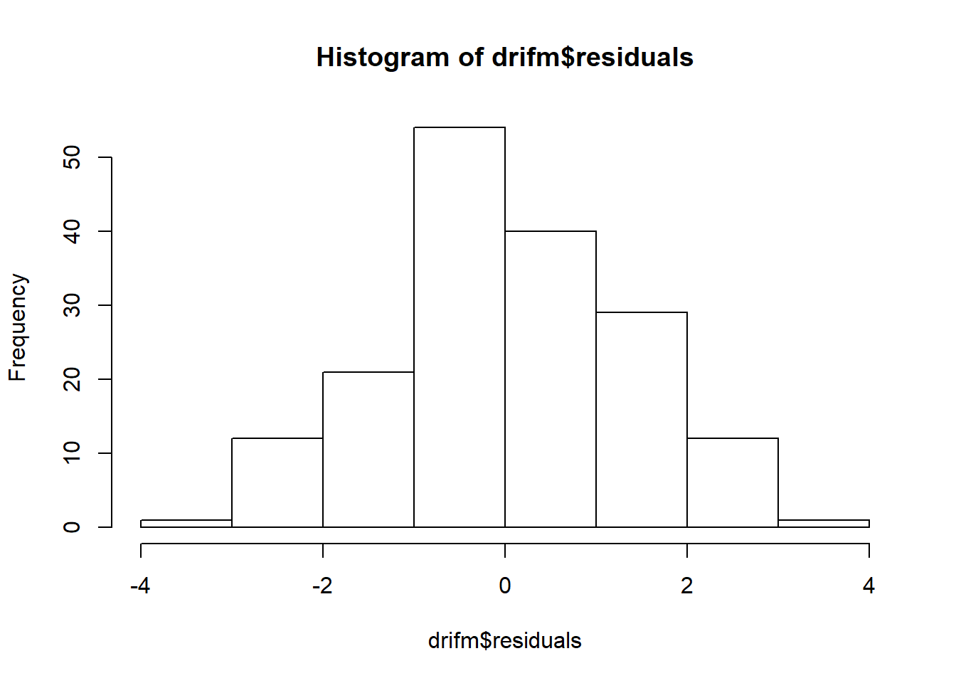
acf(driftwithoutNA) # test auto-correlation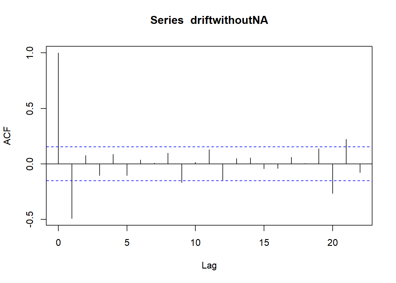
As we can see from the graph above, we have a peak at around zero and the tails to both ends look quite equal which is what would expect with the normal distribution of the residuals. From the acf() function (autocorreation function), we can test for auto-correlation: if we have several of the vertical bars above the threshold level, we have auto-correlation. Here, we can see that 4/30 bars are over/below the threshold, and that means residuals have information left in them. This means the model can be improved upon.
Autocorrelation It is a statistical term which describes the orrelation (or the ack of such) in a time series dataset. It is a key statistic because it tels us whether preovious observations infuence the recent one. It is a correlation on a time scale. If we have a random wak there are not any autocorretion. To test it we can again use the acf() function (autocorreation function) or the partia autocorreation function pacf(). Autocorreation in time series is simpy the correlation coefficient between different time points (lags) in a time series. ** Partial Autocorrelation** is the correlation coefficient abjusted for all shorter lags in a time series.
The acf() is used to identify the moving average part of the ARIMA mode, whie pacf() identifies the vaues for the autoregresiove part.
acf(lynx, lag.max = 20); pacf(lynx, lag.max = 20)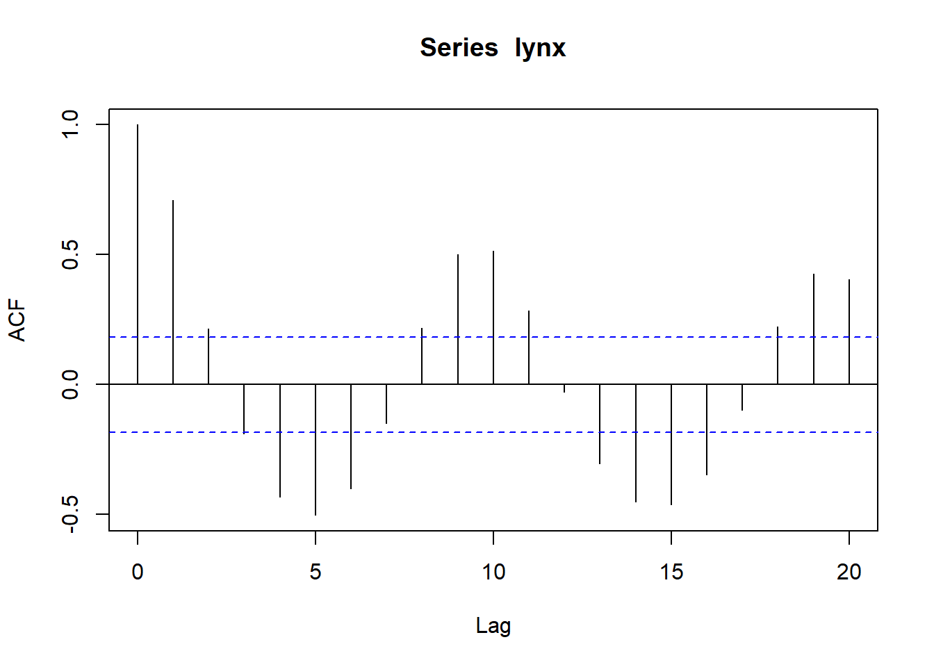

In the example above, there are sevelar bas ranging out of the 95% confidence intervals (we omit first bar because it is the autocorrelation against isef at lag0). On the contrary, pacf() starts at lag1.
Determining the Forecasting Method Quantitative forecasting can be divided in Linear: Exponential Smoothing: better in seasonaity ARIMA: better in autoregression Sesonal Decomposition: dataset needs to be seasonal (minimum number of seasonal cyces of 2) Non-Linear models: Neural Net: input is compressed to several neurons SVM: very limited in time series Clustering: aclustering approach to time series
Univariate Seasonal Time Series The main modeling oprions are: Seasonal ARIMA, Holt-Winters Exponential Smooting and Seasonal Decomposition. With Seasonal Decompositioin we divide components in trend, seasonaity and random data. This approach has several drawbacks that are: 1 - slow to catch sudden changes 2 - the model assumes that the seasonal component stays constan: this is probematic when we have ong time series where the seasona changes
It the foowing example we wi use the AirPassengers dataset to expalin the Seasonal Decomposition.
plot(AirPassengers)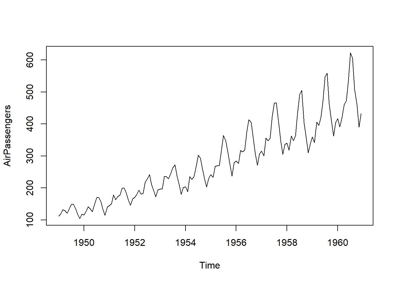
# additive mode
mymodel1 <- decompose(AirPassengers, type = "additive")
plot(mymodel1)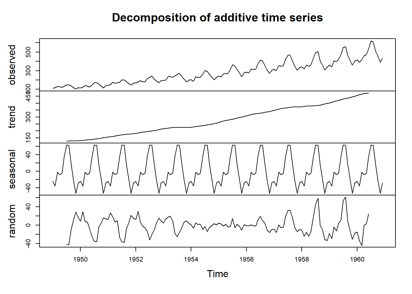
The graph shows a seasona pattern along with a trend. It is also quite evident that the seasonality increases quite a bit at the ast of the plot. The ast line of the Decomposition Graph is the random component that shows a pattern on the left and right. The middle part of the plot around 1954 and 1958 seems random, but the rest of the time series shows peaks at a certain interval. that is not a good sign and shows that the model coud be improved upon.
Exponential Smoothing with ETS It describes the time series with three parameters: Error: addictive, mutiplicative Trend: non-present, addictive, mutiplicative Seasonaity: non-present, addictive, multipicative
We can use Additive Decomposition Method that adds the Error, Trend and seasonality up. Or Mutipicative Decomposition Method that mutiplies these components. In general, if the seasona component stays constant over several cycles, it is best to use the Additive Decomposition Method. Parameters can also be mixed: additive trend with mutipicative seasonaity: that is the process of the Mutipicative Hot-Winters Mode. In Exponential Smoothing recent data is given more weight than older observations. This method has smooting coefficients to manage the weighting based on the timestamp: 1 - reactive modes relies heavly on recent data, thta results in high coefficients 2 - smooth models have low coefficients The coefficients are: alpha: initial level beta: the trend gamma: seasonality
library(forecast)
etsmodel <- ets(nottem); etsmodel
ETS(A,N,A)
Call:
ets(y = nottem)
Smoothing parameters:
alpha = 0.0392
gamma = 1e-04
Initial states:
l = 49.4597
s = -9.5635 -6.6186 0.5447 7.4811 11.5783 12.8567
8.9762 3.4198 -2.7516 -6.8093 -9.7583 -9.3556
sigma: 2.3203
AIC AICc BIC
1734.944 1737.087 1787.154 The first info we get from the results is the model type itself: ETS(A,N,A) that is about additive error, no trend and additive seasonality, that is quite what we woud expect from a temperature based data. We also see from the resuts alpha (error) and gamma (seasonaity) very closed to zero. We also see the Initial level called l = 48.92, sigma = 2.25 and three information criteria: AIC, AICc, BIC.
Let’s see how the mode looks compared to the original dataset and the forecast.
plot(forecast(etsmodel$fitted, h = 12)) # plot the forecast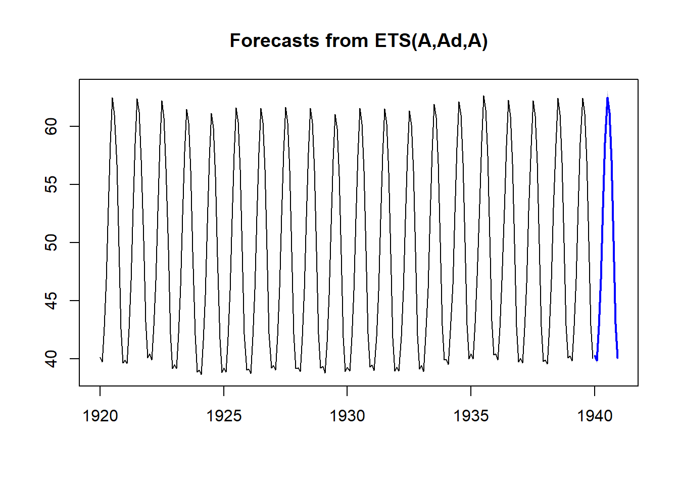 The graph gives us an extra year in blue with prediction intervals (80% accuracy and 95% accuracy). Let’s try now mutiplicative method.
etsmodmut <- ets(nottem, model = "MZM"); etsmodmutETS(M,N,M)
Call:
ets(y = nottem, model = "MZM")
Smoothing parameters:
alpha = 0.0214
gamma = 1e-04
Initial states:
l = 49.3793
s = 0.8089 0.8647 1.0132 1.1523 1.2348 1.2666
1.1852 1.0684 0.9405 0.8561 0.8005 0.8088
sigma: 0.0508
AIC AICc BIC
1761.911 1764.054 1814.121 Now, with the mutiplicative method the information criteria (AIC, AICc, BIC) are higher and that means the model is not as good as the one we got from out initially.
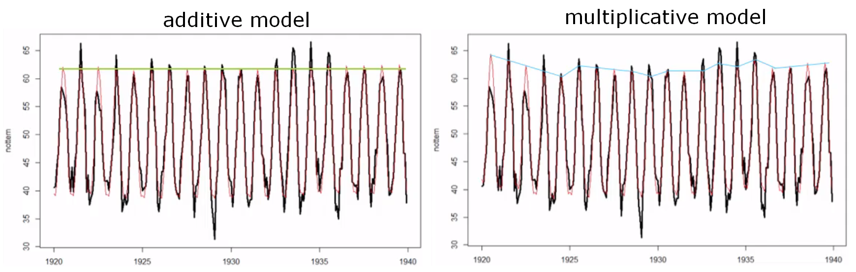
In fact, if we look at the graph comparison above, the mutiplicative method does not catch the peacks as well as the initia one. There is a big distance between the back peaks and the red peaks.
ARIMA: Autoregressiove Integrated Moving Average This is a system based on autoregression which allows to model nearly any univariate time series. It is available for univariate, and multivariate time series. ARIMA is the same of Box-Jenkins models. Generally, it is all about three parameters: p (autoregressive part): AR d (integration part, degree of differencing): I q (moving average part): MA
Crucially, the model made the time series stationary if it is not, and only then, the parameter p and q can be identified. The order of difference between the origina time series and the non-stationarity time series is described by the d parameter.
The all ARIMA model is based on the summation of lags (autoregressive part) and the summation of the forecasting error (moving average part). For example: ARIMA(2,0,0) is a second order (lag) of autoregressive parameter AR and we are interested in the first and second lag. For the first order autoregressive AR(1) or ARIMA(1,0,0) we have the formuation:
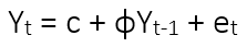
The observed value Yt at time point t consist of the constant c plus the value of previous time point (t-1) multiplied by a coefficient ɸ plus the error term of time point t (et). For the forecasting the Kalman Filter would be applied in order to the error term.
ARIMA(0,1,0) means the time series is not constant, which is required for a forecast. We are not in presence of stationarity (dataet with no constant mean). The differencing is:
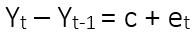
The formua above says that the present observation Yt minus the preavious observation Yt-1 is equal to a constant plus an error term. The term t-1 is also called the Backshift Operator which is used to denote differencing time series.