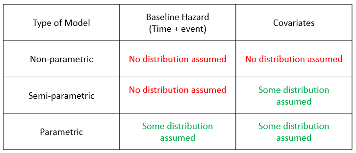
There are differences between Parametric Models (e.g. Kaplan-Meier), Semi-Parametric Models (e.g. Cox Proportional Hazard), and Non-Parametric Models. The graph below gives the main pieces of information. A survival analysis can be defined as consisting of two parts: the core survial object with a time indicator plus the corresponding event status (used to calculate the baseline hazard). The second part of the survival model consists of the covariates. We have to keep in mind that both of these parts can have a different distributions, or it is totally possible that no distribution at all is assumed.
There are many distributioin and these distributions have different probability patterns in hisogram depending on th fiel of reseach. For example, in economics a Pareto distribution is often used to described the wealth situation in a given society. It is a fairly good way to show if a large chunk of money is owned by just a small amount of people. In survival analysis, there is not a clear cut, there are a few of commonly used. Mainly the Exponential Distribution as well of the Weibull Distribution are common choices.
Prostate Cancer Dataset We will use as a template for survival analysis the prostate cancer dataset. The dataset come from a study on prosthetic cancer patients, and it contains several variables to indicate or are in correlation with prosthetic cancer. The data contain 63 patients and 8 independent variables. The main goal is to compare two different treatments identified with 1 or 2. Both ot these are surgical treatments which are pretty much indicative in higher stages of prostate cancer. The two tretments 1 and 2 differ in the amount of removed tissue and the type of tisue it was primarily removed. The time in the dataset was measured in months. The variable status can be 0=censoring (loss of follow up or quitting the study), or 1=no censoring. The variable sh is the blod measurement hormone. The variable size is the tumor size at the beginning of the study. The variable index is the Gleason Scoring System, because tumor has different stages and they actually start to metastasize other boby parts at higher index of Gleason Scoring System.
prost <- read.table("C:/07 - R Website/dataset/TS/prostate-cancer.txt", header = FALSE)

colnames(prost) = c("patient", "treatment", "time", "status", "age", "sh", "size", "index")
head(prost)
patient treatment time status age sh size index
1 1 1 65 0 67 13.4 34 8
2 2 2 61 0 60 14.6 4 10
3 3 2 60 0 77 15.6 3 8
4 4 1 58 0 64 16.2 6 9
5 5 2 51 0 65 14.1 21 9
6 6 1 51 0 61 13.5 8 8# Parametric model
library(flexsurv)
weib_mod <- flexsurvreg(Surv(time, status) ~ treatment + age + sh + size + index, data=prost, dist = "weibull")
exp_mod <- flexsurvreg(Surv(time, status) ~ treatment + age + sh + size + index, data=prost, dist = "exp")
plot(weib_mod) # weibull curve
lines(exp_mod, col="blue")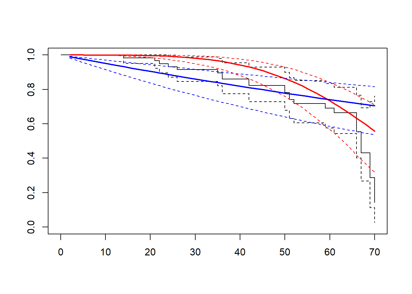
The idea behind the Exponential distribution is that the probability of an event is exactly the same at any time point. On the other hand, in the very popular Gaussian normal distribution it is assumed that most of events take place somewhere around the mean of the survival curve. The Weibull distribution allows us to set the time point on the survival curve where most of the events will take place. This is especially interesting when we have a situation where the events take place mostly at the end of the study. For example, the longer a person lives, the higher the probability of death will be. For humans this is expecially true after 70 years of life.
From the graph above, the black line is a classic step plot of the survival object. Essentially, the black line is a Kaplan-Meier plot which we can easly comapre against the red line which is our fit of the Weibull based survival curve. From the red line, we can see that at the beginning the line is more like a flat line, and this is because of the nature of the Weibull distribution, where the event probability is assumed to be higher at the end than at the beginning. In blue we have the line of the exponential distribution which is a constant slope, in fact, the underlying assumption for exponential distribution is a constant probability of events throughout the whole serie. This assumption is often not a good fit in survival analysis. In fact, we can see from the graph above the discrepancy between the Keplan-Meier and the blue line. That is not a good sign and proves that the Weibull curve is a much better fit for this dataset.