An hazard rate is the probability estimate of the time it takes for an event to take place. The event can be anything ranging from death of an organism or failure of a machine or any other time to event setting. There are external factors that influence the probabililty of an event, covariates. For example: how many miles was the car used or did the owner exchange the oil regularly. The proportional hazards model allows us to incorporate thse covariance into our model, and it makes th probability estimate much more accurate. In Medical Setting covariance cold be for example: gender, age, weight, occupation, treatment, other diseases. In Engineering Setting covariance coul be age, material, construction, environment, frequency of usage.
The assumption of the Cox Proportional Hazards Model is possible to estimate the effect of the beta parameters without any consideration of the hazard function. In fact, David Cox observed that if the proportional hazards assumption holds, then it is possible to estimate the beta effect parameters without any consideration of the hazard function. The data should be stationalry and constant over time.
Prostate Cancer Dataset We will use as a template for survival analysis the prostate cancer dataset. The dataset come from a study on prosthetic cancer patients, and it contains several variables to indicate or are in correlation with prosthetic cancer. The data contain 63 patients and 8 independent variables. The main goal is to compare two different treatments identified with 1 or 2. Both ot these are surgical treatments which are pretty much indicative in higher stages of prostate cancer. The two tretments 1 and 2 differ in the amount of removed tissue and the type of tisue it was primarily removed. The time in the dataset was measured in months. The variable status can be 0=censoring (loss of follow up or quitting the study), or 1=no censoring. The variable sh is the blod measurement hormone. The variable size is the tumor size at the beginning of the study. The variable index is the Gleason Scoring System, because tumor has different stages and they actually start to metastasize other boby parts at higher index of Gleason Scoring System.
prost <- read.table("C:/07 - R Website/dataset/TS/prostate-cancer.txt", header = FALSE)

colnames(prost) = c("patient", "treatment", "time", "status", "age", "sh", "size", "index")
head(prost)
patient treatment time status age sh size index
1 1 1 65 0 67 13.4 34 8
2 2 2 61 0 60 14.6 4 10
3 3 2 60 0 77 15.6 3 8
4 4 1 58 0 64 16.2 6 9
5 5 2 51 0 65 14.1 21 9
6 6 1 51 0 61 13.5 8 8# Cox Proportional Hazard
library(survival)
cox <- coxph(Surv(time, status) ~ treatment + age + sh + size + index, data =prost)
summary(cox)Call:
coxph(formula = Surv(time, status) ~ treatment + age + sh + size +
index, data = prost)
n= 63, number of events= 23
coef exp(coef) se(coef) z Pr(>|z|)
treatment -0.69695 0.49810 0.53471 -1.303 0.1924
age -0.08361 0.91979 0.03692 -2.265 0.0235 *
sh -0.23664 0.78927 0.18511 -1.278 0.2011
size 0.06786 1.07021 0.02833 2.395 0.0166 *
index 0.77410 2.16865 0.18803 4.117 3.84e-05 ***
---
Signif. codes: 0 '***' 0.001 '**' 0.01 '*' 0.05 '.' 0.1 ' ' 1
exp(coef) exp(-coef) lower .95 upper .95
treatment 0.4981 2.0076 0.1747 1.4206
age 0.9198 1.0872 0.8556 0.9888
sh 0.7893 1.2670 0.5491 1.1345
size 1.0702 0.9344 1.0124 1.1313
index 2.1686 0.4611 1.5002 3.1350
Concordance= 0.866 (se = 0.037 )
Likelihood ratio test= 38.4 on 5 df, p=3e-07
Wald test = 26.47 on 5 df, p=7e-05
Score (logrank) test = 34.47 on 5 df, p=2e-06The interpretation of the results above is to look at the matrix of covariance with the coefficients and significant indicators. In our case, we have the variables age, size and index that are significant expecially the index variable is important for the model. using these information we can potentially eliminate the les significant variable and simplify the model. At the bottom of the result, we can see the Concordance (0.866). It is the probability of the agreement for any teo randomly chosen obsrvations. It tells us the chance of being correct in selecting the one observation with a higher risk of an event. We want a concordance close to one. Any concordance lower than 0.5 is a vary bad model. The last statistics is the Likelihood ratio test. It is the fraction of variance in the survival rate that is predicted from the covariance. If the p-values are significant, then we might reject the null hyppothesis and assume that the covarince do have an influence on the survival rate. The degrees of freedom in these tests are equivalent to the amount of covariance in the model.
# Plot the model
library(ggfortify)
autoplot(survfit(cox))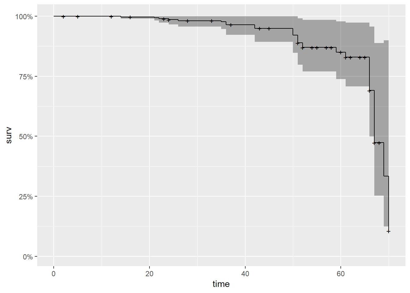
As we can see from the graph above, it is quite similar to the Kaplan-Meier generated curve. The survival probability drops dramatically after around 75 months.
Aalen’s Additive Regression Model There is one more thing to keep in mind with covarince. The influence of covariates might vary depending on the time point within the study. In our prosthetic cancer study, it is absolutely possible that a large tumor size does not influence the sirvival probability for one or two years at the beginnig of the study. But after that time period, a large tumor can become a huge burden and highly lower the sirvival chances. In order to model the time dependent effect of covariates we have the Aalen’s Additive Regression Model.
# Define and Plot the Aalen model
aalen<- aareg(Surv(time, status) ~ treatment + age + sh + size + index, data =prost)
autoplot(aalen)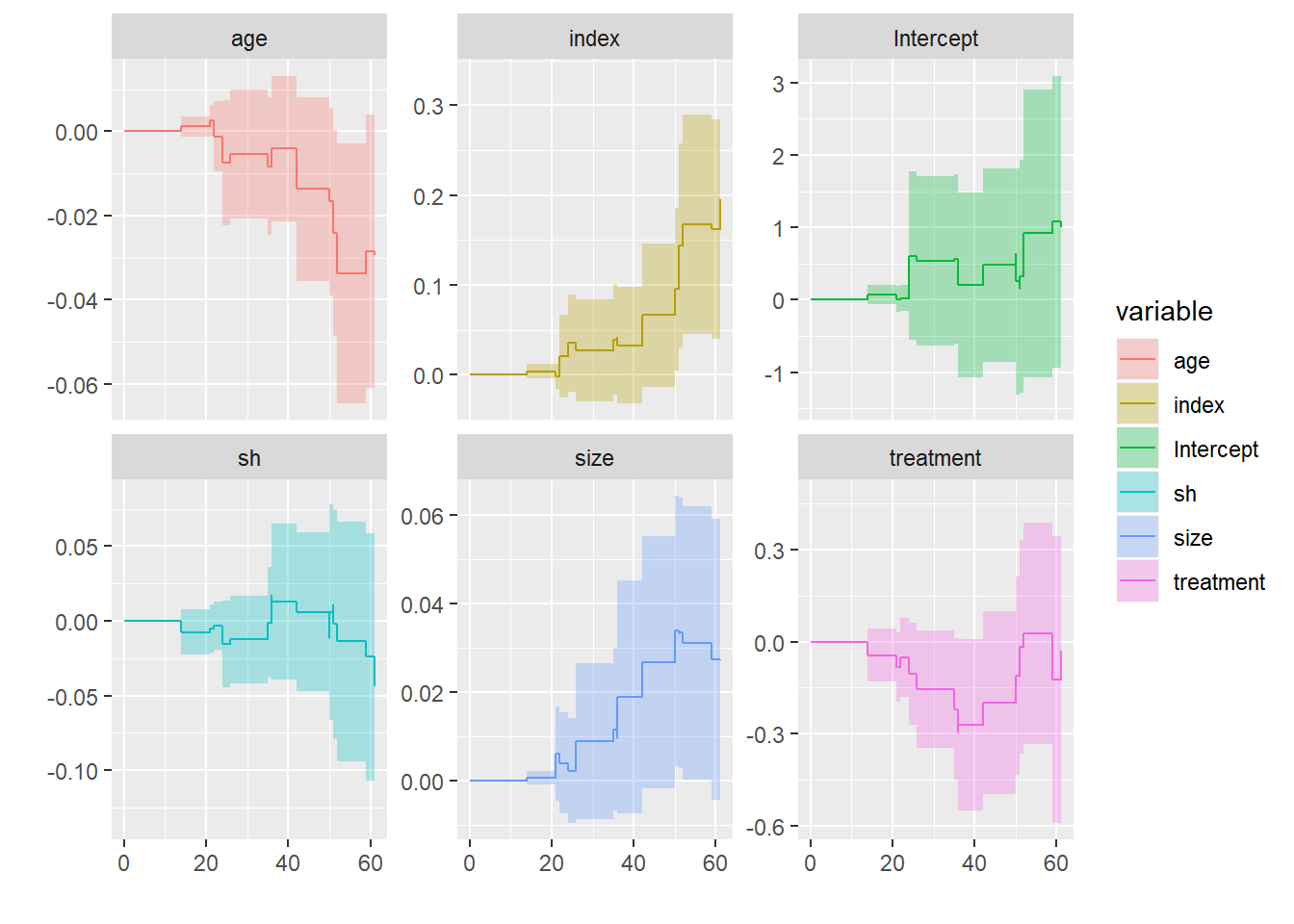
If we check out the plot sheet above, we can indeed see that the tumor size and tumor index have an increasing effect on the hazard rate. That means the longer a subject with a large tumor or a high tumor index, the more influential these covariance actually get. In other words we can say that at the beginning of the study the sizeand the index are not that important. But after some years this changes in subjects that do have a large tumor or a high index scorand they are more likely to die. The opposite effect can be seen that higher age can be benefial after some time in th study.