In this particular field R is favored over Python. In fact, R has more features for Time Series. A precious resource is the Rob Hyndman’s Blog. It explains step by step the standard univariate time series analysis.
FIRST TRENDING DATA In this example we explore how many people are working in a country: unemployment rate vs. labor force participation rate. That is used for propaganda purposes, because low unemployment rates show an optimistic picture about the economics of a country. This is very easy to manipulate. On the contary, the Labor Force Participation Rate is harder to manipulate: it calculate the percentage of people in the work force vs. available people of a particular age range. In this example the Age range is between 25 to 54 years.
singapur <- c(70.19999695, 71.09999847, 71.69999695, 72.30000305, 73.09999847, 72.90000153, 74.40000153, 75.40000153, 76, 76.90000153, 77.40000153, 78.19999695, 78.90000153, 78.69999695, 79, 78, 80, 79.80000305, 80.30000305, 80.5, 80.69999695, 81.09999847, 81.5, 81.90000153, 82.30000305, 82.69999695, 83.19999695, 83.5)
# Convert to time series
singapur <- ts(singapur, start = 1980)
plot(singapur, ylab = "Labor Force Participation Rate")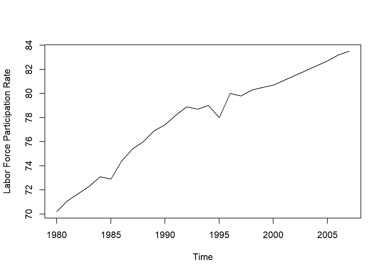 The graph above show us that it is clarly trending dataset with increasing values over a time span of 30 years. The biggest problem we have to keep in mind is the fact that this is a rate, and the values cannot be higher than 100%. Therefore, we need a threshold for linear trend, because otherwise the model would go to infinity. This method is the Linear Trend Model with Damping parameter. Now we explore how to handle time series with trend, and which methods are available for that, and how to avoid pitfalls.
EXPONENTIAL SMOOTING MODEL This family of models includes: Simple Exponantial Smoothing Holt’s Linear Trend Model Holt-Winters Seasonal Method Automated Exponantial Smoothing
Because the data wewe are dealing have not seasonality, we canuse the Hold Linear Trend Model. The idea behind the hold linear trend is as follow:
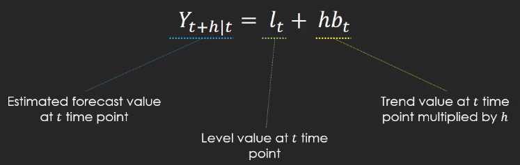
Note, that b is the trend value of the time series. In Exponential Smoothing the equation is adjusted to the fact the data is sensible to only recent data or not. This is a very responsive model that can be influenced by the last few observations or on older data. We have to adjust the model using the alpha parameter (level) and beta (trend). The parameter gamma here is omitted because we have not seasonality. The closer the beta smoothing parameter is to one, th more the model relies on the latest values. On the contrary, when the parameter is close to zero, would produce a more smooth model with even the older data being taken into consideration.
Lets to implement the Hold Linear Trend Model.
library(forecast)
holttrend = holt(singapur, h = 5) # forecast 5 years
summary(holttrend)
Forecast method: Holt's method

Model Information:
Holt's method

Call:
 holt(y = singapur, h = 5)

  Smoothing parameters:
    alpha = 0.6378
    beta  = 0.1212

  Initial states:
    l = 69.619
    b = 0.6666

  sigma:  0.5529

     AIC     AICc      BIC
65.79969 68.52697 72.46072

Error measures:
                      ME      RMSE       MAE        MPE      MAPE
Training set -0.08247984 0.5118728 0.3084414 -0.1056525 0.3986079
                  MASE        ACF1
Training set 0.5047223 -0.09190023

Forecasts:
     Point Forecast    Lo 80    Hi 80    Lo 95    Hi 95
2008       83.90071 83.19216 84.60926 82.81708 84.98435
2009       84.28751 83.39799 85.17703 82.92711 85.64791
2010       84.67431 83.58796 85.76065 83.01289 86.33573
2011       85.06111 83.76361 86.35860 83.07676 87.04545
2012       85.44790 83.92606 86.96975 83.12045 87.77536
plot(holttrend)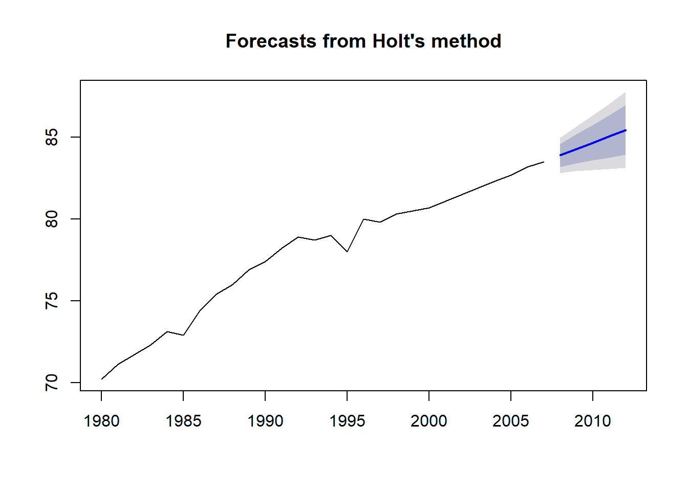
In the summary we have a lot of crucial information about the model. We get the values of alpha (0.63) and beta (012). This indicates that the trend which is basically the slope of the time series plot is fairly constant. In fact, the graph above shows in blue the forecast the values from 2008 to 2012 and it shades the confidence interval of 80 and 95 percent. From the forecast, we see that the trend line follow the trand of the period 1998 and 2007. Before 1998, there is a brief period of stagnation, and before this period there was an yearly increase even steeper.
Looking again from the summary results, we see Initial states: these are the value of the slope and the level value. Then, we have the information criteria and the error measures. Keep in mind that we are dealing with rate values and they can not exceed 100%, that is qhy the trend sooner or later the forecast will encounter a flat trend closed to 100%. We have to incorpurate this assumption using the Dumpt Argument inside our function. Dampt is also named phi parameter: phi close to 1: the forecast is close to the original slope of the Hold trend model phi close to 1: the forecast trend will be flattened very soon In pratice, the phi is set between 0.8 and 0.95.
plot(holt(singapur, h = 15, damped = TRUE, phi = 0.85)) # damped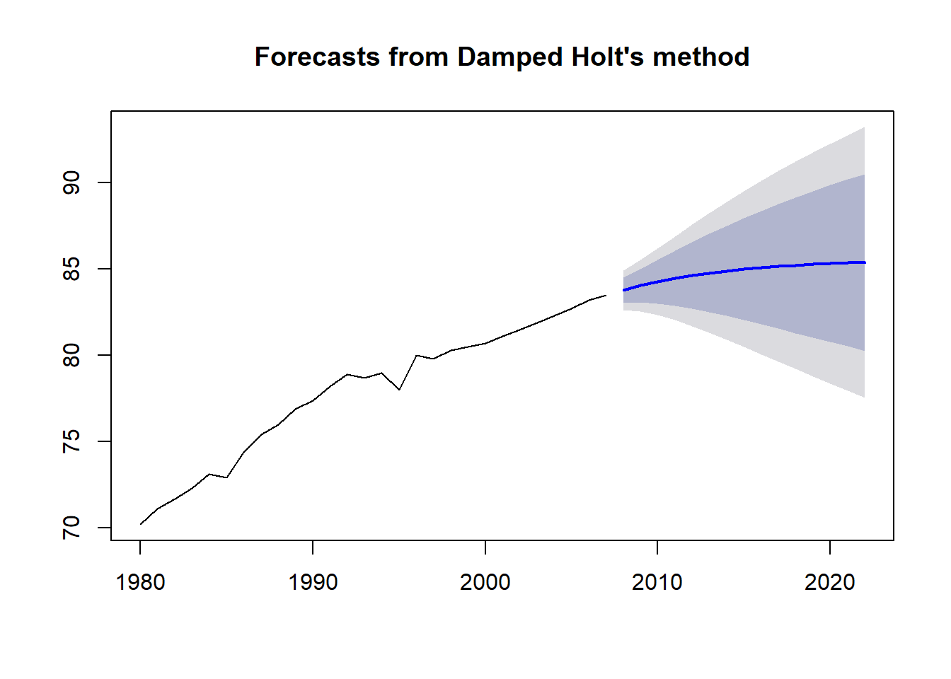
The graph above, shows the forecast with the dampter parameter, and clearly shows a curve that is more round and get flat at the end of the trajectory.
ARIMA MODEL The ARIMA model is also known as Box-Jenkins model are a standard modeling system for time series. This method is composed by: AR: AutoRegressive, and this meands seasonality and trend. In R is called P. I: Integration, used to suppress the dataset differences between the oservations and the original values, eliminating portion of chaos in the dataset. In R is called D. MA: Moving Average: moviment around a constant mean. In R is called Q.
The Autocorrelation AR says that we have to deal with trending data. This means that an observation at an earlier time point influences the later observations.
singapurarima <- auto.arima(singapur)
summary(singapur)
Min. 1st Qu. Median Mean 3rd Qu. Max.
70.20 75.15 78.80 77.92 80.80 83.50 plot(forecast(singapurarima, h = 55))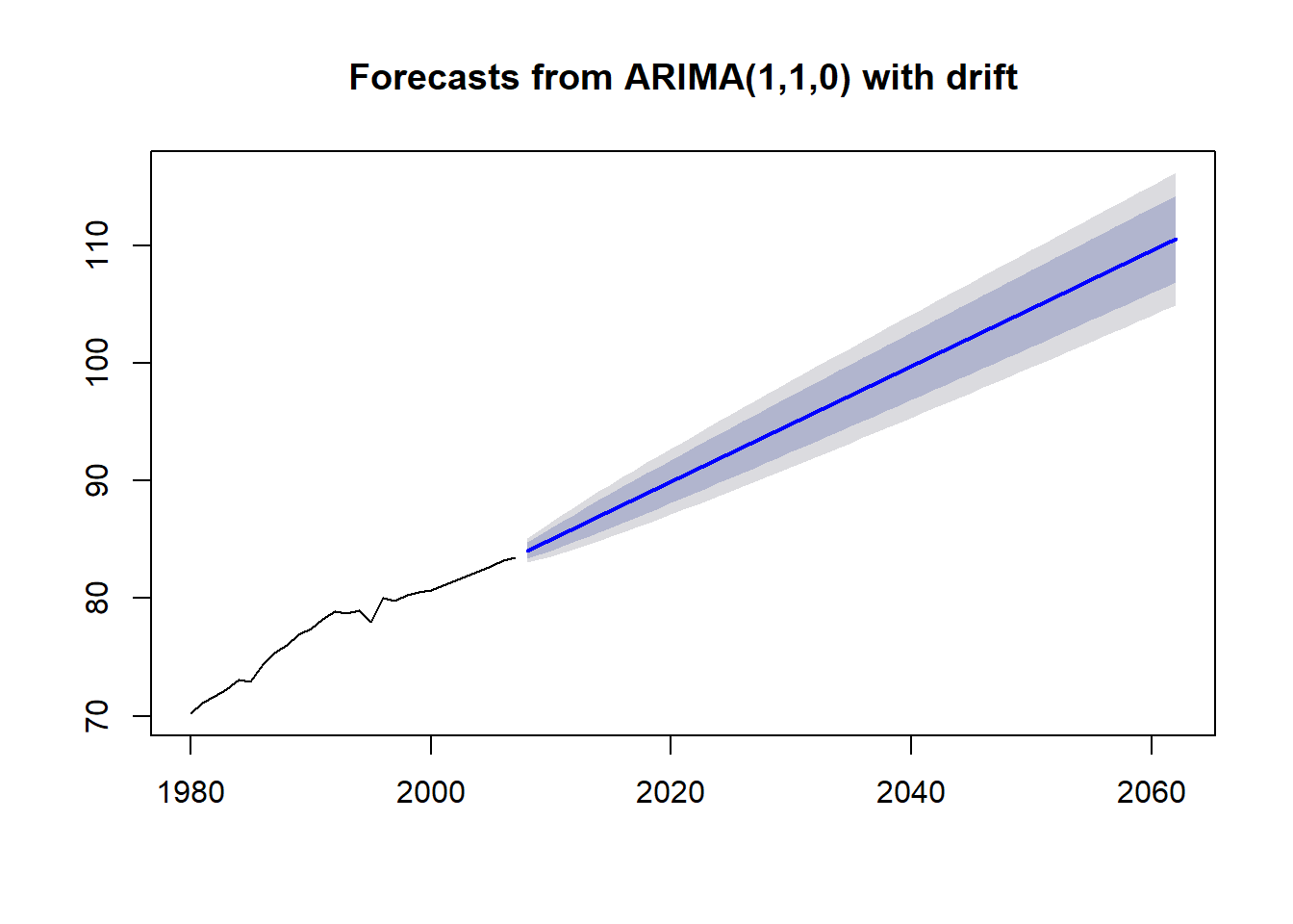
As we can see from the graph above, this set up of the ARIMA model work fine on a short time span, but on a longer time span we would be skeptical due to the fact that overcome the 100% value. There is a little trick to avoid this error, and consists to inactivate the stepwise parameter and approximation in order to get more accurate model.
COMPARISON OF THE MODELS A huge part of statistics it is the visualization of the results. Humans are primarily visual, therefore this is the fastest and best way to explain a model to a broad audience.
holttrend <- holt(singapur, h = 10)
holtdamped <- holt(singapur, h = 10, damped = TRUE)
arimafore <- forecast(auto.arima(singapur), h = 10)

library(ggplot2)
autoplot(singapur) +
  forecast::autolayer(holttrend$mean, series = "Holt Linear Trend") +
  forecast::autolayer(holtdamped$mean, series = "Holt Damped Trend") +
  forecast::autolayer(arimafore$mean, series = "ARIMA") +
  xlab("year") + ylab("Labour Force Participation Rate Age 25-54") +
  guides(colour=guide_legend(title="Forecast Method")) + theme(legend.position = c(0.8, 0.2)) +
  ggtitle("Singapur") + theme(plot.title=element_text(family="Times", hjust = 0.5, color = "blue", face="bold", size=15))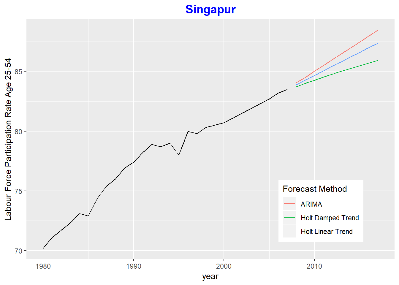
The graph above shows the original dataset on the left side in black and the right side of the plot shows the fprecasted lines for the three models we discussed in our example. The Hold Linear Model is the most conservative, which tends towards the lowest rate in the future. The ARIMA Model is the most aggressive model with highest projected rates.
SECOND SEASONAL DATA In this example, we use the Inflation rate: a measure of change in purchasing power per unit of money. On top of that, it is important to know how the inflation moves since it directly affects investment opportunities. Prices of stocks, precious metals or oil are at least indirectly affected by the rate of inflation. In this example, we use the German Inflaction rate from 2008 to 2017.
mydata <- c(-0.31, 0.41, 0.51, -0.20, 0.61, 0.20, 0.61, -0.30, -0.10, -0.20, -0.51, 0.41,
-0.51, 0.61, -0.20, 0.10, -0.10, 0.30, 0.00, 0.20, -0.30, 0.00, -0.10, 0.81,
-0.60, 0.40, 0.50, 0.10, -0.10, 0.00, 0.20, 0.10, -0.10, 0.10, 0.10, 0.60,
-0.20, 0.60, 0.59, 0.00, 0.00, 0.10, 0.20, 0.10, 0.20, 0.00, 0.20, 0.19,
-0.10, 0.68, 0.58, -0.19, 0.00, -0.19, 0.39, 0.38, 0.10, 0.00, 0.10, 0.29,
-0.48, 0.57, 0.48, -0.47, 0.38, 0.09, 0.47, 0.00, 0.00, -0.19, 0.19, 0.38,
-0.56, 0.47, 0.28, -0.19, -0.09, 0.28, 0.28, 0.00, 0.00, -0.28, 0.00, 0.00,
-1.03, 0.85, 0.47, 0.00, 0.09, -0.09, 0.19, 0.00, -0.19, 0.00, 0.09, -0.09,
-0.84, 0.38, 0.75, -0.37, 0.28, 0.09, 0.28, 0.00, 0.09, 0.19, 0.09, 0.74,
-0.64, 0.65, 0.18, 0.00, -0.18, 0.18, 0.37, 0.09, 0.09, 0.00)
germaninfl <- ts(mydata, start = 2008, frequency = 12)
plot(germaninfl)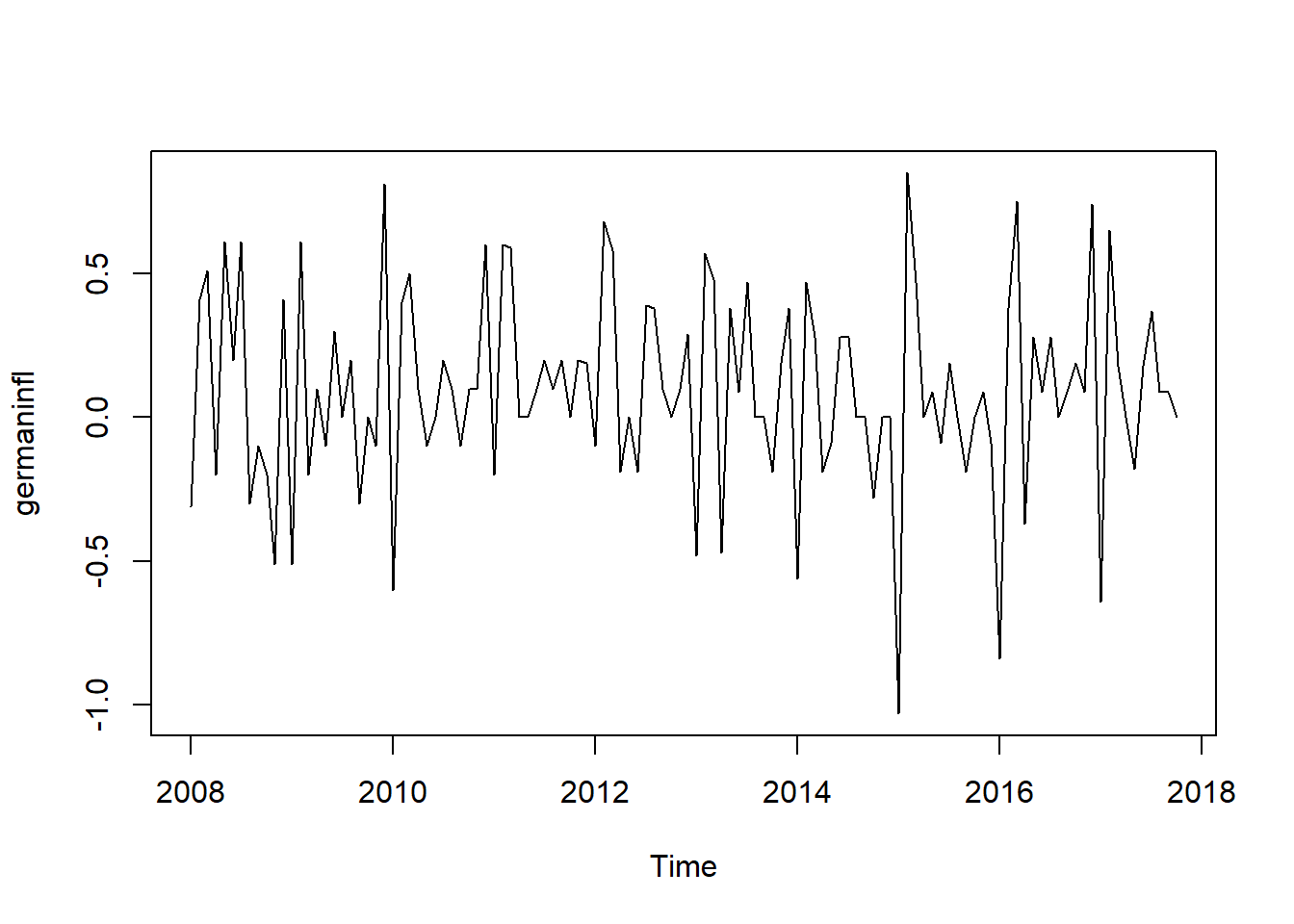 From the graph above, we can see several important facts about the dataset. First and foremost,this dataset has not trend, the mean stays constant over the whole series. Second, this dataset is seasonal, and so, seasonal decomposition comes into play here if at least there are more than two seasonal cycles. The Seasonal ARIMA and Exponatial Smooting can work with this sort of data. But we have to start with the Seasonal Decomposition. We also need to use Cross Validation.
In this example we focused on Seasonality and Cross Validation. Cross validation is used to estimate the accuracy of a model and find which is the best model that better fit for the seasonal data we are dealing with. There is a significant difference between a time series with and without seasonality.
We first start with Seasonal Decomposition. With this method we dividing the data into its compnents: trend, seasonality and white noise. There are some drawbacks of seasonal decompsition: First few values are NA Slow to catch fast rises Assumes a constant seasonal component
We start to use the EXPONANTIAL SMOOTING METHOD.
plot(stl(germaninfl, s.window = 7))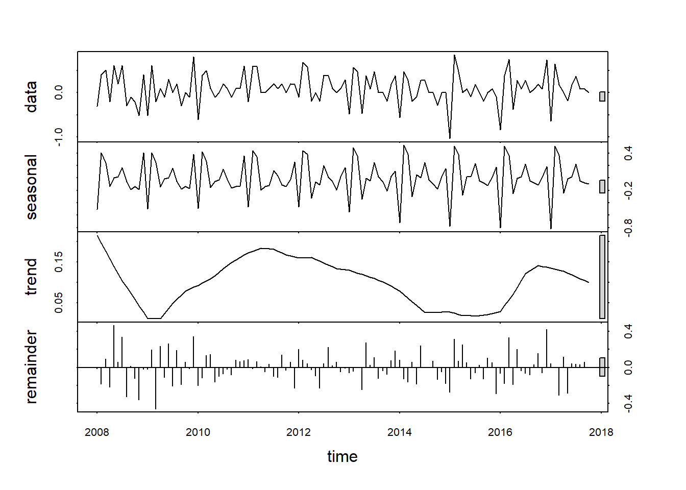
library(ggplot2)
autoplot(stlf(germaninfl, method = "ets"), h = 24) # method for the forecasting is the ets: exponential smoothing method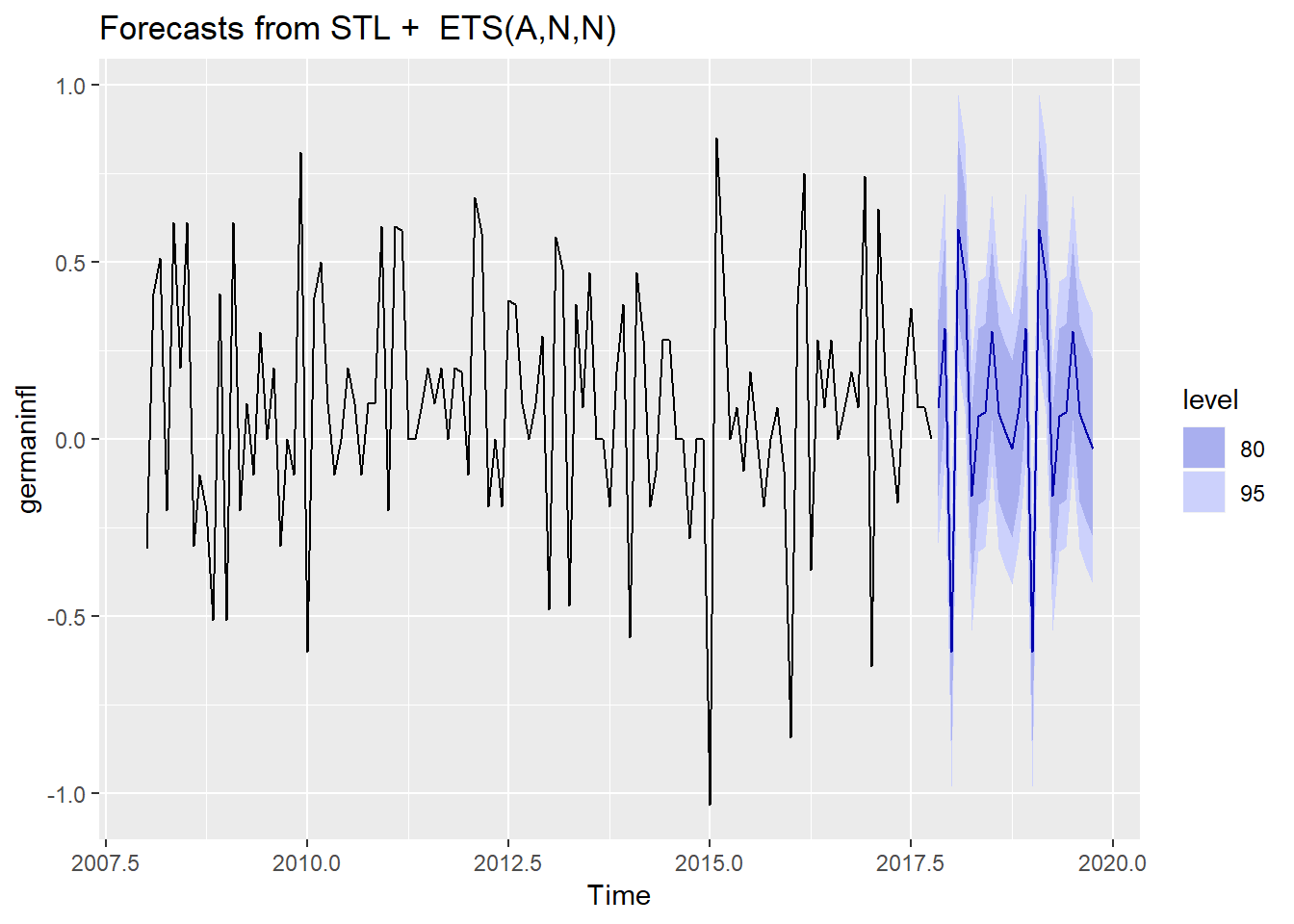
The graph above shows that there is not trend in the series. The whole trend component makes a half circular move from 2009 to 2015, and starts to rise again in late 2016. Overall there is not a clear trend direction. The interest part is the seasonal component. The series starts with a low January inflaction which is instantly compensated for the February. We have another inflaction spike in the middle of the year which might be the holiday season and then we get to Christmas time with high inflaction. This make perfect sense because during the holiday and Christmas are time of great consumption, and retailers tend to adjust the prices.
As an alternative, we can use SEASONAL ARIMA MODEL. the main difference between an Seasonal ARIMA and Non Seasonal ARIMa model is that in Seasonal ARIMA we have a set of seasonal parameters.
germaninflarima <- auto.arima(germaninfl, stepwise = TRUE,
           approximation = FALSE, trace = TRUE)
 ARIMA(2,0,2)(1,1,1)[12] with drift         : Inf
 ARIMA(0,0,0)(0,1,0)[12] with drift         : 31.97975
 ARIMA(1,0,0)(1,1,0)[12] with drift         : 22.54641
 ARIMA(0,0,1)(0,1,1)[12] with drift         : 6.801819
 ARIMA(0,0,0)(0,1,0)[12]                    : 29.92568
 ARIMA(0,0,1)(1,1,1)[12] with drift         : Inf
 ARIMA(0,0,1)(0,1,0)[12] with drift         : 29.30375
 ARIMA(0,0,1)(0,1,2)[12] with drift         : Inf
 ARIMA(0,0,1)(1,1,2)[12] with drift         : Inf
 ARIMA(1,0,1)(0,1,1)[12] with drift         : 1.682708
 ARIMA(1,0,0)(0,1,1)[12] with drift         : 6.386517
 ARIMA(1,0,2)(0,1,1)[12] with drift         : 0.04883016
 ARIMA(2,0,3)(0,1,1)[12] with drift         : 2.305377
 ARIMA(1,0,2)(0,1,1)[12]                    : -2.165703
 ARIMA(1,0,2)(1,1,1)[12]                    : Inf
 ARIMA(1,0,2)(0,1,0)[12]                    : 20.35976
 ARIMA(1,0,2)(0,1,2)[12]                    : Inf
 ARIMA(1,0,2)(1,1,2)[12]                    : Inf
 ARIMA(0,0,2)(0,1,1)[12]                    : 2.269403
 ARIMA(2,0,2)(0,1,1)[12]                    : -0.729167
 ARIMA(1,0,1)(0,1,1)[12]                    : -0.4490938
 ARIMA(1,0,3)(0,1,1)[12]                    : -0.3068147
 ARIMA(0,0,1)(0,1,1)[12]                    : 4.749057
 ARIMA(2,0,3)(0,1,1)[12]                    : Inf

 Best model: ARIMA(1,0,2)(0,1,1)[12]
forec <- forecast(germaninflarima)
plot(forec)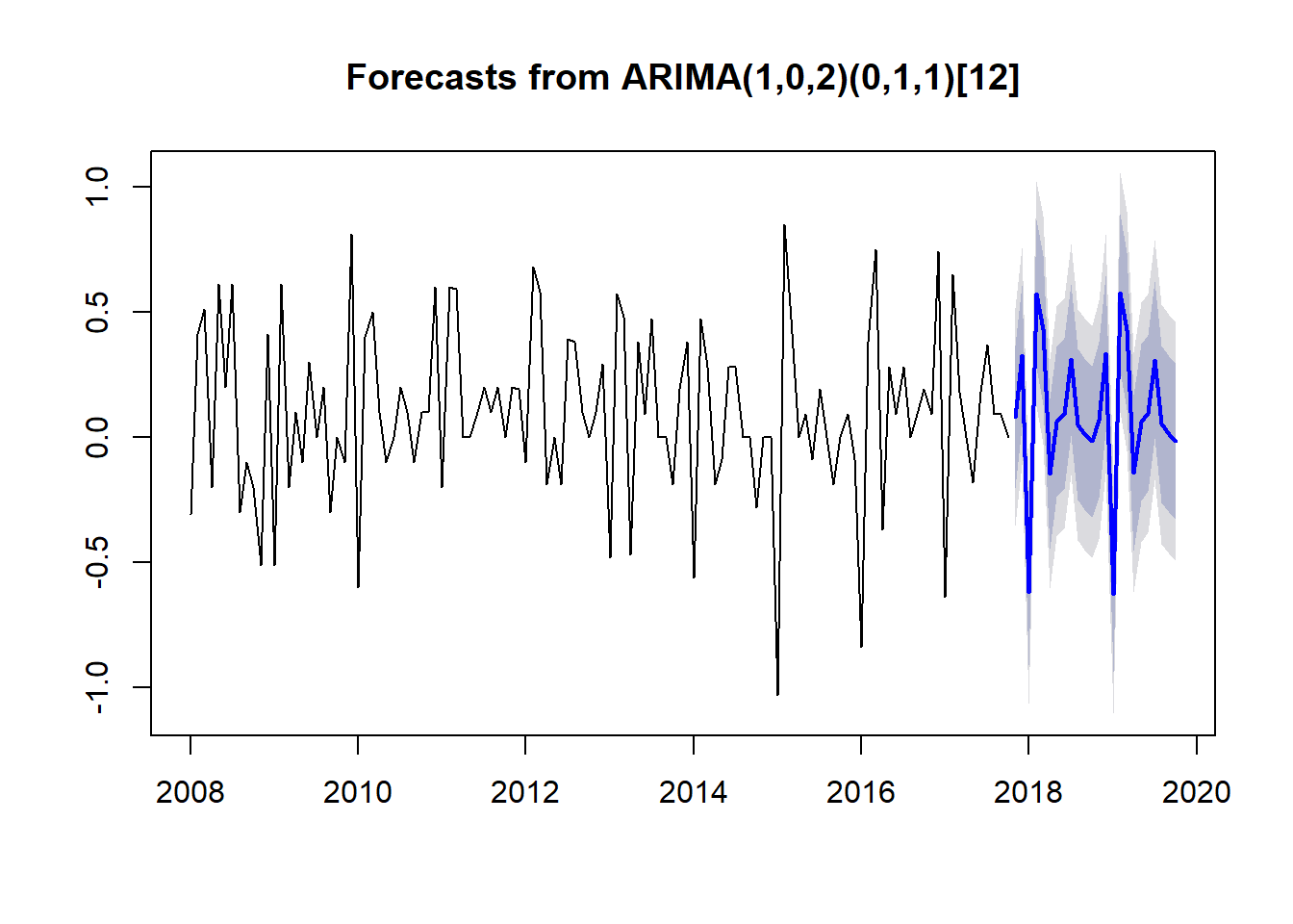
The auto.arima() function has calculated the following model: ARIMA(1,0,2)(0,1,1)[12]. The corrisponding coefficient are the ar2: autoregressiove coefficient for the non-seasonal part, and ma1, ma2: moving average one and two for non-seasonal, then we have the sma1: seasonal moving average for the seasonal part. The parameter [12] says that we have an annual frequency.
Now, we try to compare Time Series model using the Cross Validation method. It is not a good idea to only use the Information Criteria like AIC and BIC, because ARIMA and Exponential Smooting cannot be compared just with Information Criteria, because the underlying statistics used to calculate the information criteria are different for both models systems. We have to focus on Forecast Accuracy like Mean Squared Error MSE that produce an error rate for each time point in the series. The time series is splitted in Training and Test set. The Test set is only one observation and the Training set is all the data before the Test set. That means, the error rates are computed one oafter another and along the timeline. This is called the Rolling Forecast Origin. Then, we comapre the error rate of the two models (the difference bewteen the forecasted and actual values). We can use the Root Mean Squared Error RMSE or the Mean Squared Error MSE. This approach is more legant that the classical Training 80% - Test 20% approach.