This article is a summary of the StatQuest video made by Josh Starmer. Click here to see the video explained by Josh Starmer.
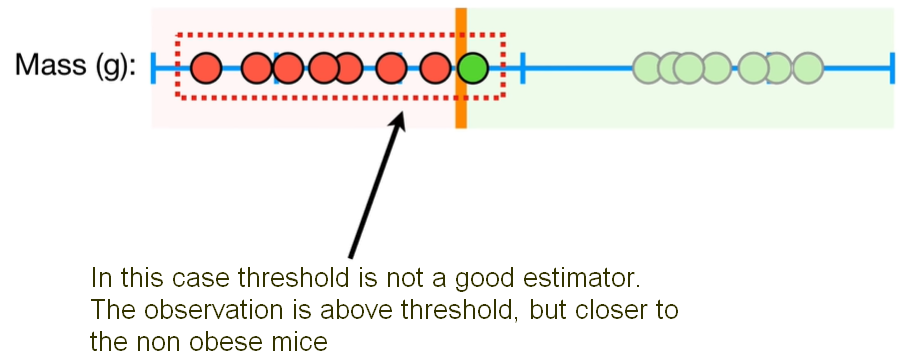
We use as an example the measurement of the Mass of mice (g). The red dots in the figure below represent mice that are not obese and the green dots represent mice obese. Based on this observation, we can pick a threshold, and when we have a new observation that has less mass than the threshold we can classify it as not obese. And when we have a new observation with more mass than the threshold we can classify it as obese. However, when we have a new observation just above the threshold we classify it as obese, but it doesn’t make a lot of sense, because the observation is much closer to the not obese observations, as depicted in the figure here below. So, this threshold is pretty lame.
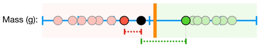
To solve this problem, we can focus on the observations on the edges of each cluster and use the midpoint between them as the threshold called Maximal Margin Classifier. Now, with this method, the same observation we considered before is closer to the not obese mice than iti is to the obese mice. So, it makes sense to classify this observation as not obese.
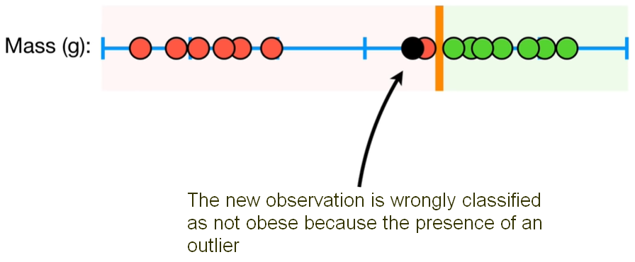
But actually, the Maximal Margin Classifier is not the best solution to classify our mice. If fact we could have an outlier observation that was classified as not obese (i.e. big mouse not obese), but was much closer to the obese observation. In this case the Maximal Margin Classifier would be super close to the obese observation and relly far from the majority ot the not obese mice. So, Maximal Margin Classifier is super sensitive to outliers. See figure below.
To make a threshold that is not so sensitive to the outliers we must allow misclassification. Choosing a threshold that allows misclassifications (we not take in consideration outliers) is an example of Bias/Variance Tradeoff that plagues all of machine learning. When we allow misclassification, the distance between the observations and the threshold is called a Soft Margin. To find the best Soft Margin we use Cross Validation to determine how many misclassifications (outliers) and observations to allow inside the Soft Margin to get the best classification. When we use a Soft Margin to determine the location of a threshold, then we are using a Soft Margin Classifier aka a Support Vector Classifier to classify observations.
The name Support Vector Classifier comes from the fact that the observations on the edge and within the Soft Margin are called Support Vectors.
Now, if each observation has not only the Mass (g) measurement but also the Height (cm) measurement, then the data would be two-dimensional; in this case the Support Vector Classifier is a line. The blue parallel lines in the figure below give us a sense of all of the other points are in relation of the Soft Margin (i.e. we have one not obese observation inside the soft margin and it is missclassified). Just like before, we use Cross Validation that allow us to find better classification. In mathematics jargon, a line is a Flat affine 1-Dimensional subspace.
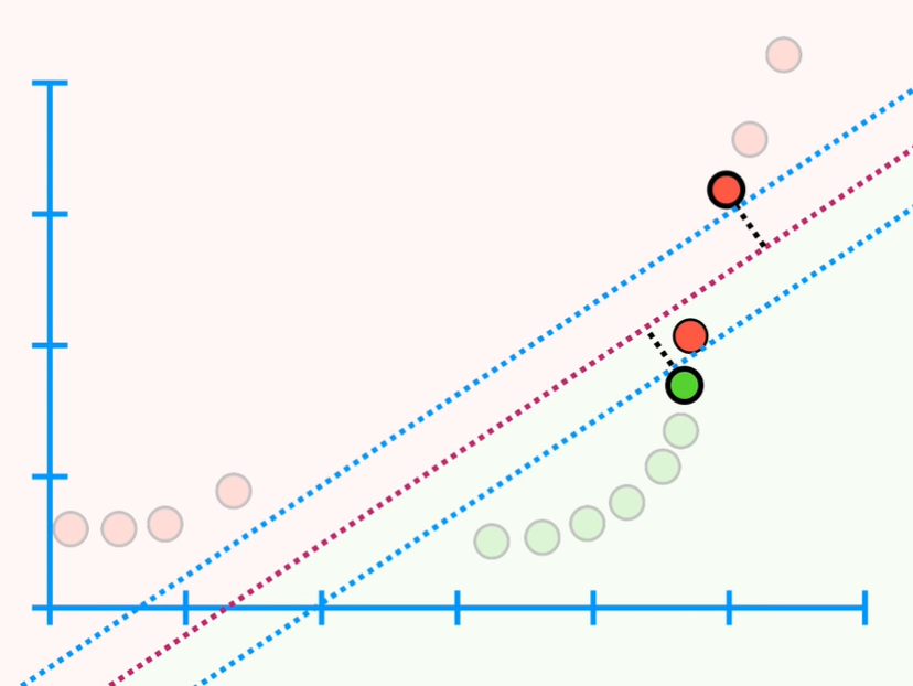
From the figure above we can see that we have one observation inside the soft margins and it is misclassified. Just like before, we use Cross Validation that allow us to find better classification for the misclassified observation. Moreover, if we have three dimensions the support vector classifier is a plane instead of a line. And we classify new observations by determining which side of the plane they are on. In mathematics jargon, a line is a Flat affine 2-Dimensional subspace. When the data are in 4 or more dimensions, the Support Vector Classifier is a Hyperplane, and in mathematics jargon a hyperplane is a Flat affine subspace.
Very High Overlapping - Support Vector Machine Support Vector Classifier seems very good because it can handle outliers and overlapping classifications. But what can happen when we have tons of overlapping? For example, consider that we are looking at Drug Dosages where red dots in the figure below are people not cured and in green dot people cured.
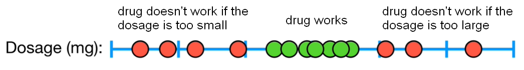
With the high overlapping depicted above, no matter where we put the classifier because will always make a lot of misclassifications. So, Support Vector Classifiers don’t perform well with this type of data. The solution is to use the Support Vector Machines. We use the x-axis which represent the dosages we observed, but we also add an y-axis that will be the square of the dosages.
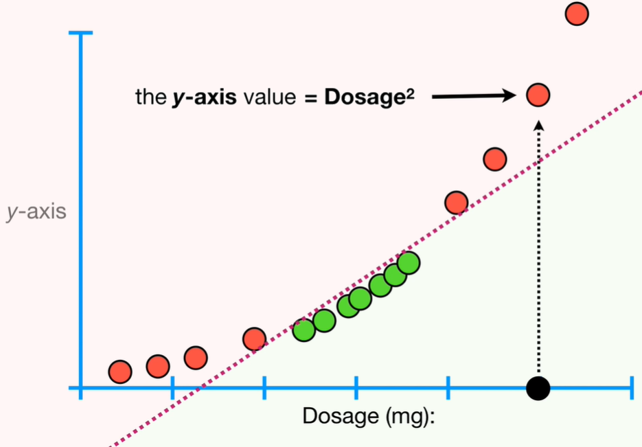
The main idea behind Support Vector Machines are: 1 - start with data in a relatively low dimension (in this example one dimension dosage in mg) 2 - move the data into a higher dimension (in this example from one to two dimensions) 3 - find a Support Vector Classifier that separates the higher dimensional data into two groups
Kernel Function How do we decide how to transform the data in the y-axis? In order to make the mathematics possible, Support Vector Machines use something called Kernel Function to systematically find Support Vector Classifiers in higher dimensions. In our example we use the Polynomial Kernel, which has a parameter d which stands for the degree of the polynomial, and this polynomial is used to find the Support Vector Classifier. When we have d=3 we would get a 3rd dimension based on dosage that result in a plane, again used to find the Support Vector Classifier. In summary, the Polynomial Kernel increases dimensions by setting d as the degree of the polynomial. We can use Cross Validation to find the best value of d.
A very commonly used Kernel is the Radial Kernel, also known as the Radial Basis Function Kernel - RBF. The closest observations (aka the nearest neighbors) have a lot of influence on how we classify the new observation, and observations that are further away have relatively little influence on the classification.
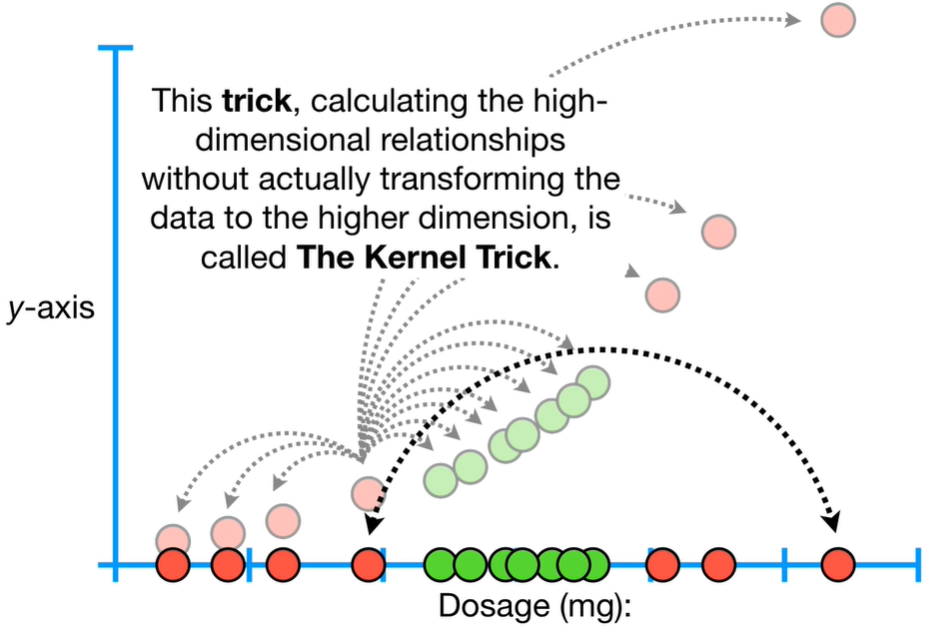
The Kernel Functions only calculate the relationships between every pair of points as if are in the higher dimensions. This trick, calculating the high-dimensional relationships without actually transforming the data to the higher dimension, is called The Kernel Trick. The Kernel Trick reduces the amount of computation required for Support Vector Machine by avoiding the math that transforms the data from low to high dimensions.