Random Forest is a Bagging process of Ensemble Learners. Random Forests are built from Decision Tree. Decision Trees work great, but they are not flexible when it comes to classify new samples. It creates a bootstrapped dataset with the same size of the original, and to do that Random Forest randomly selects rows with replacement. After creating a bootstrap dataset, it creates a decision tree using the bootstrapped dataset, but using only a subset of variables at each step. So, it builds a tree using bootstrapped dataset, and only considering a Random Selection of Variables. Random Forest ideally repeats these two steps 100 times, that result in a wide variety of trees making Random Forest more effective than the Individual Decision Tree.
data <- read.csv("C:/07 - R Website/dataset/ML/CTG.csv")
data$NSP <- as.factor(data$NSP)
table(data$NSP)
   1    2    3
1655  295  176
We are using a dataset of 2126 observations and 22 variables, and the data we use is called CTG data and it containes measurement of fetal heart rate FHR and uterine contraction UC features on cardiotocograms. CTGs was classified by three expert obstetricians, and classification label are: Normal, Suspect, or Pathologic. The response variable is NSP Fetal State Class Code (1=Normal, 2=Suspect, 3=Pathologic) as we can see from the table above.
# Data Partition
set.seed(123)
ind <- sample(2, nrow(data), replace = TRUE, prob = c(0.7, 0.3))
train <- data[ind==1,]
test <- data[ind==2,]

# Random Forest
library(randomForest)
set.seed(456)
rf <- randomForest(NSP~., data=train,
                   ntree = 300,       # number of trees
                   mtry = 8,          # number of variables tried at each split
                   importance = TRUE,
                   proximity = TRUE)
print(rf)
Call:
 randomForest(formula = NSP ~ ., data = train, ntree = 300, mtry = 8,      importance = TRUE, proximity = TRUE)
               Type of random forest: classification
                     Number of trees: 300
No. of variables tried at each split: 8

        OOB estimate of  error rate: 5.48%
Confusion matrix:
     1   2   3 class.error
1 1137  18   5  0.01982759
2   47 165   1  0.22535211
3    6   5 111  0.09016393
# Using attribues we can see and than explore al the attribute of RM, for example
# writing: rf$confusion we can see the confusion matrix of our model
# attributes(rf)From the resul above, we can see we used 300 number of trees and 8 variables at each split (typically is the squared root of the number of variables). The Out of the Bag OBB estimated error rate is 5.75% which is quite good, because it means we have around 95% of accuracy. About the Out of the Bag OBB we have to remember that we allowed replacement entries: that means some rows were not included, typically about one third of the original data, does not end up in the bootstrapping sample. This sample is call: Out of Bagging dataset. We can use the Out of Bagging dataset as a Test Set and look if most of the bootstrapped trees correctly classify the Out of the Bag dataset. We do the same for all the rows of the Out of the Bag dataset. The Error in Classification is called: Out of the Bag Error. Looking at the Confusion Matrix above we can see that the prediction is quite good when predictiong Class 1 (Normal) with a class.error of 1.7%. On the contrary there is a class.error of 12.23%% when predicting Class 3 (Pathologic). Using the function attribues() we can see and than explore al the attribute of RM, for example writing rf$confusion we can see the confusion matrix of our model.
# Prediction & Confusion Matrix - train data
library(caret)
p1 <- predict(rf, train)
confusionMatrix(p1, train$NSP)
Confusion Matrix and Statistics
Reference
Prediction 1 2 3
1 1160 2 0
2 0 211 0
3 0 0 122
Overall Statistics
Accuracy : 0.9987
95% CI : (0.9952, 0.9998)
No Information Rate : 0.7759
P-Value [Acc > NIR] : < 2.2e-16
Kappa : 0.9964
Mcnemar's Test P-Value : NA
Statistics by Class:
Class: 1 Class: 2 Class: 3
Sensitivity 1.0000 0.9906 1.00000
Specificity 0.9940 1.0000 1.00000
Pos Pred Value 0.9983 1.0000 1.00000
Neg Pred Value 1.0000 0.9984 1.00000
Prevalence 0.7759 0.1425 0.08161
Detection Rate 0.7759 0.1411 0.08161
Detection Prevalence 0.7773 0.1411 0.08161
Balanced Accuracy 0.9970 0.9953 1.00000# # Prediction & Confusion Matrix - test data
p2 <- predict(rf, test)
confusionMatrix(p2, test$NSP)Confusion Matrix and Statistics
Reference
Prediction 1 2 3
1 481 18 4
2 13 60 2
3 1 4 48
Overall Statistics
Accuracy : 0.9334
95% CI : (0.9111, 0.9516)
No Information Rate : 0.7845
P-Value [Acc > NIR] : <2e-16
Kappa : 0.8109
Mcnemar's Test P-Value : 0.3514
Statistics by Class:
Class: 1 Class: 2 Class: 3
Sensitivity 0.9717 0.73171 0.88889
Specificity 0.8382 0.97268 0.99133
Pos Pred Value 0.9563 0.80000 0.90566
Neg Pred Value 0.8906 0.96043 0.98962
Prevalence 0.7845 0.12995 0.08558
Detection Rate 0.7623 0.09509 0.07607
Detection Prevalence 0.7971 0.11886 0.08399
Balanced Accuracy 0.9050 0.85219 0.94011# Error rate of Random Forest
plot(rf)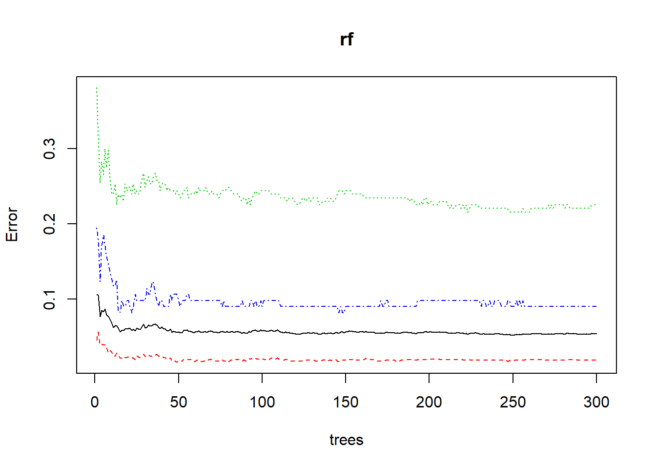
From the result above we can see the confusion matrix of the train and test set, and also Sensitivity and Spesificity for each of the three classes. We have a mismatch because the OOB error rate is 5.75%, but the Accuracy is 99.87%. We have to remeber that OBB is the Out of the Bag estimator, and so is not in the bootstrap sample. The solution of the mismatch is that the Accuracy s based on the train set and not on the OOB. Form the Error Rate Plot above we can see that as the number of trees grows the OBB (on the y-axis) intially il high and then, it become constant. In fact the graph says that it is not necessary to use more than 300 number of trees.
Now we can try to tune the paramenters of our model.
# Tune mtry
t <- tuneRF(train[,-22], train[,22], # esclude the response variable
       stepFactor = 0.5,             # per each interations number of variables tried at each split (mtry) in inflated by 0.5
       plot = TRUE,                  # plot OOB
       ntreeTry = 300,               # tuning number of trees
       trace = TRUE,
       improve = 0.05)               # it is the relative improvement in OOB error and so the improvement of the RM depends on the 0.05
mtry = 4 OOB error = 5.62%
Searching left ...
mtry = 8 OOB error = 5.02%
0.1071429 0.05
mtry = 16 OOB error = 5.42%
-0.08 0.05
Searching right ...
mtry = 2 OOB error = 6.82%
-0.36 0.05 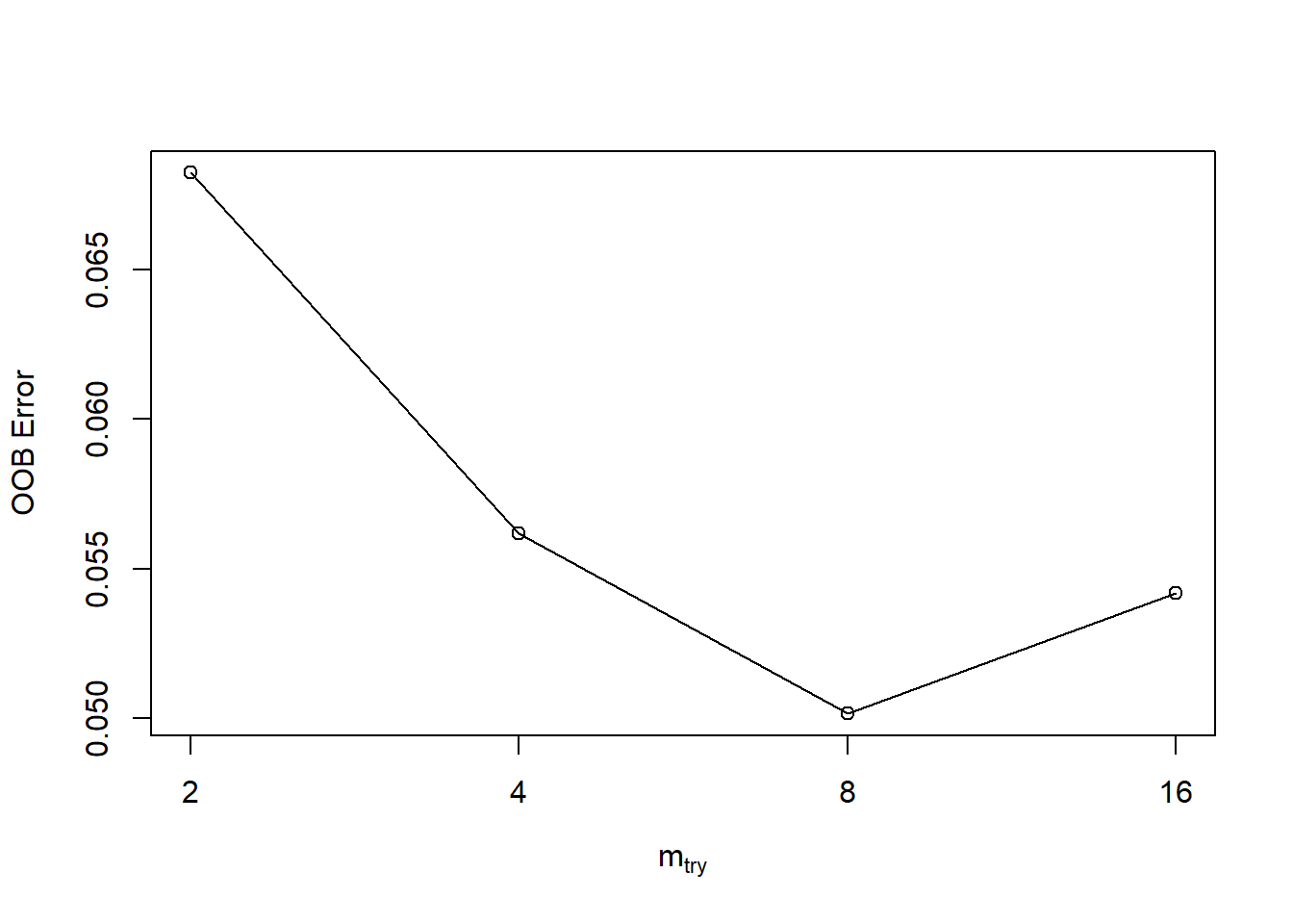
# Number of nodes for the trees
hist(treesize(rf),                        # give us the number of trees in term of number of nodes
     main = "Number of Nodes for the Trees",
     col = "grey")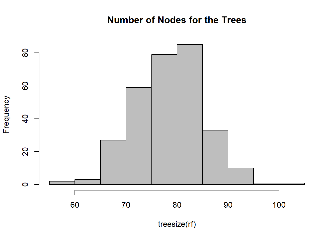
# Variable Importance
varImpPlot(rf,
           sort = T,
           n.var = 10,
           main = "Top 10 Variable Importance")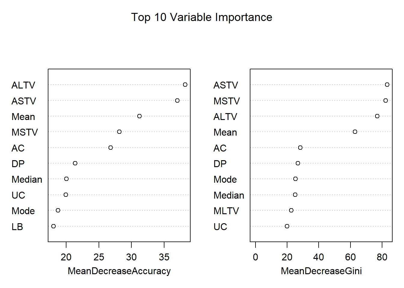
# Quantitative values of Variable Importance
# importance(rf)

# Find out how many times the predictor variables are actually used in the random forest
# varUsed(rf)
From the first of the three graphs that we have above OOB Error Graph we can see that OOB Error is initially high (0.07), and then it comes down when we use as number of variables tried at each split mtry of 4 and even better with mtry of 8. On the contrary, when mtry is equal to 16, the OOB Error start to increase again. With this graph, now we have a better understanding about which value of number of variables tried at each split mtry to use. We used 300 trees in our model, and the second graph that we have here above is an histogram about the distribution of number of nodes in our 300 trees that we used. There are 80 trees that contain 80 nodes, and there are also few trees with 60 nodes or 100 nodes. From the last of the three graph above, we can see which of the variables are the most important in the model. The first graph on the left tests how worse the model performs without each variable using the Mean Decrease Accuracy. We can see for example that the variable DS has a contribution closed to zero. The second graph on the right measures how pure the nodes are at the end of the tree without each variable, using the Mean Descease Gini. We can aslo use the function varUsed(rf) to find out how many times the predictor variables are actually used in the random forest.
Now we use the Partial Dependence Plot in order to have a graphical representation of the marginal effect of a variable on the call probability.
# Partial Dependence Plot
partialPlot(rf, train, ASTV, "1") # use ASTV variable and test it for class 2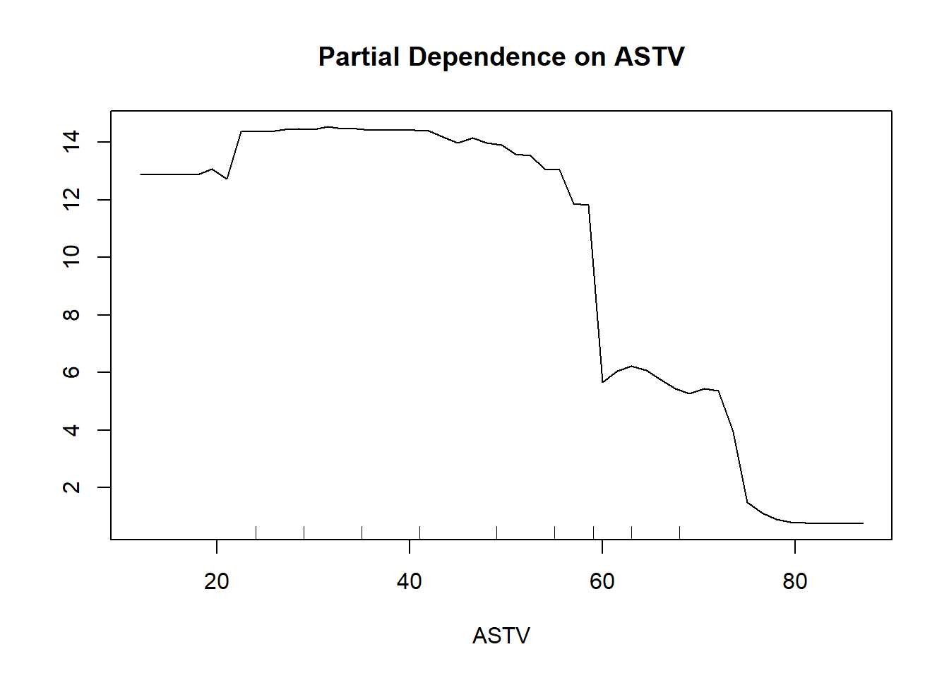
# Extract Single Tree
# getTree(rf, 1, labelVar = TRUE)

# Multi-dimensional Scaling Plot of Proximity Matrix
MDSplot(rf, train$NSP)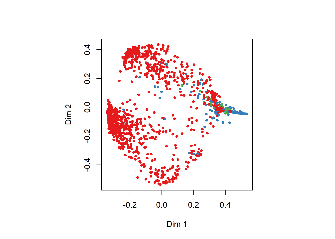
From the Partial Dependence Plot above made for the variable ASTV at class 1 Normal, we can see that when the variable ASTV is less than 60, the model tend to predict class 1 more strongly compare when ASTV is more than 60.
We can extract Information about the Single Tree using the function getTree(rf, 1, labelVar = TRUE) where in this example we specify we want the first tree in our Random Forest. From the output, not shown here, when we get in the variabe status the value -1, this means that we get a terminal node, and so we have also the corresponding value of the class inside the varible prediction.
We can also use the Multi-dimensional Scaling Plot for dimension 1 Dim1 and dimension 2 Dim2. The colors are related to the threelevel of the response variable NSP Fetal State Class Code (1=Normal, 2=Suspect, 3=Pathologic). The dimensions Dim1 and Dim2 imply the variation in data along the two principal components.