Linear Discriminant Analysis

Linear Discriminant Analysis was originally developed by R.A. Fisher to classify subjects into one of the two clearly defined groups. It was later expanded to classify subjects inoto more than two groups. It helps to find linear combination of original variables that provide the best possible separation between the groups.
Linear Discriminant Analysis is focused on maximizing the separability among known categories. The problem is when 2 features are not sufficient to capture the most of variation. In PCA, we solve this problem reducing the dimensionality by focusing on the feature with the most variation. LDA is like PCA, but is focused to maximize the separability between the two groups. PCA is unsupervised, but LDA is supervised.

data(iris)

library(psych)
pairs.panels(iris[1:4],
             gap = 0,
             bg = c("red", "green", "blue")[iris$Species],
             pch = 21)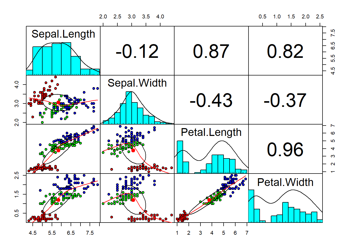

We are using the iris dataset with 4 numerical variables and 1 factor which has 3 levels as described above. We can also see that the numerical variables have different ranges, it is a good pratice to normalize the data.
From the graph above we have scatterplots of each combination of variabels. In the upper triangle we have correlation coefficients. We can see that Sepal.Length and Petal.Length are good to separate between thr three Species. In other cases, there is a overlapping and not a clear separation between the three Species.

# Data Partitioning
set.seed(123)
ind <- sample(2, nrow(iris),
              replace = TRUE,
              prob = c(0.6, 0.4))

training <- iris[ind==1,]
testing <- iris[ind==2,] 

# Linear Discriminant Analysis
library(MASS)
linear <- lda(Species~., data=training)
linear

Call:
lda(Species ~ ., data = training)

Prior probabilities of groups:
    setosa versicolor  virginica 
 0.3370787  0.3370787  0.3258427 

Group means:
           Sepal.Length Sepal.Width Petal.Length Petal.Width
setosa         4.946667    3.380000     1.443333    0.250000
versicolor     5.943333    2.803333     4.240000    1.316667
virginica      6.527586    2.920690     5.489655    2.048276

Coefficients of linear discriminants:
                    LD1         LD2
Sepal.Length  0.3629008  0.05215114
Sepal.Width   2.2276982  1.47580354
Petal.Length -1.7854533 -1.60918547
Petal.Width  -3.9745504  4.10534268

Proportion of trace:
   LD1    LD2 
0.9932 0.0068 

From the resul above we have the Coefficients of linear discriminants for each of the four variables.
The first discriminant function LD1 is a linear combination of the four variables: (0.3629008 x Sepal.Length) + (2.2276982 x Sepal.Width) + (-1.7854533 x Petal.Length) + (-3.9745504 x Petal.Width). Note that Discriminant functions are scaled. We have aslo the Proportion of trace, the percentage separations archived by the first discriminant function LD1 is 99.32%.

Now we can create a Stacked Histogram of Discriminant Function values.

# Histogram
p <- predict(linear, training)
ldahist(data = p$x[,1], g = training$Species) # p$x[,1] give data from LD1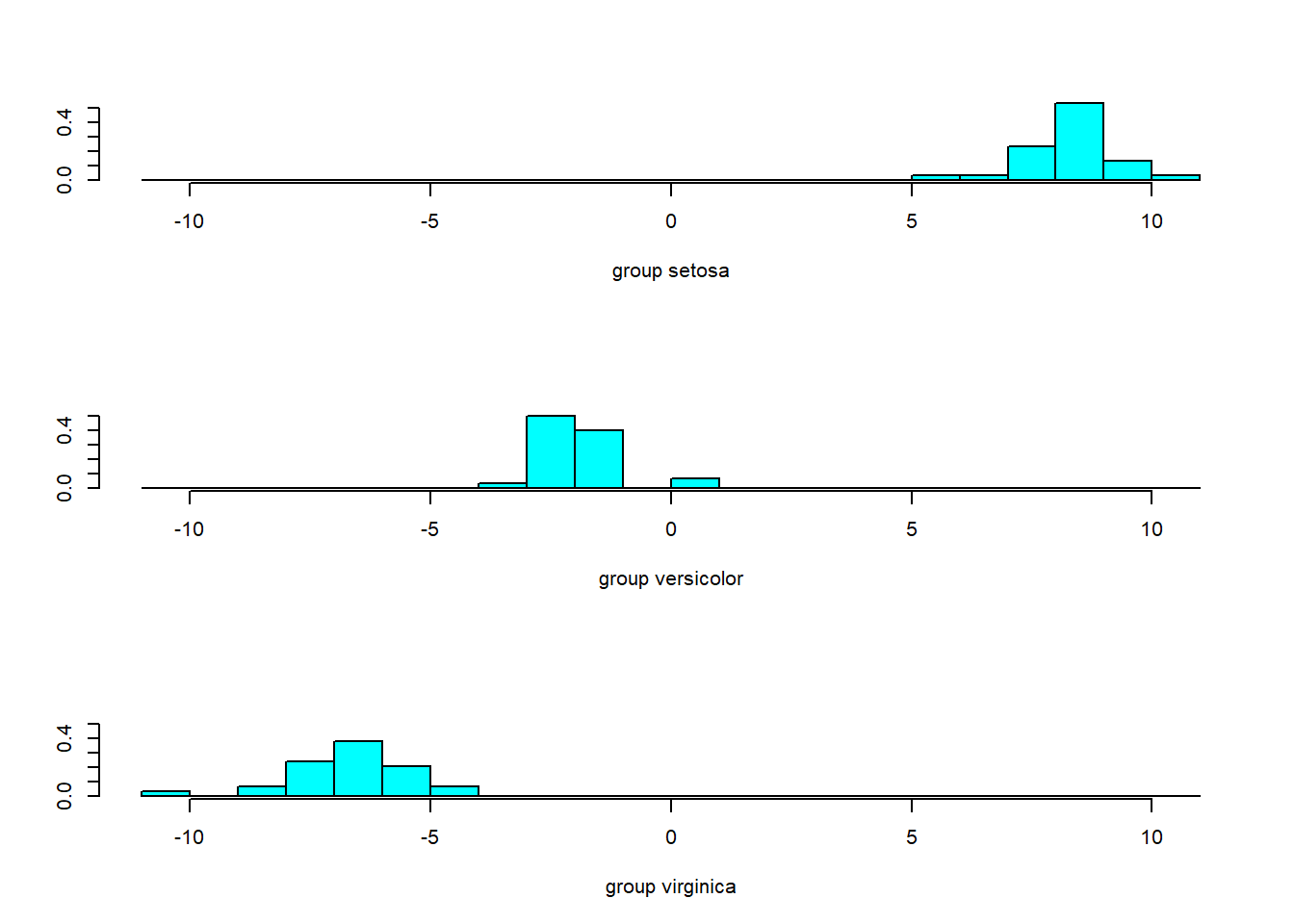

From the graph above, we have histogram from LD1, and w can see that the separatin between setosa and the oder two Species is quite large with no overlap. On the contrary, there is a certan amont of overlapping between versicolor and virginica. We already said that the percentage of separation archived by LD1 is 99.32%, that is we he can see a very clear separation from the histogram above. Now, we can try to do the same for LD2.

# Histogram
p <- predict(linear, training)
ldahist(data = p$x[,2], g = training$Species) # p$x[,1] give data from LD1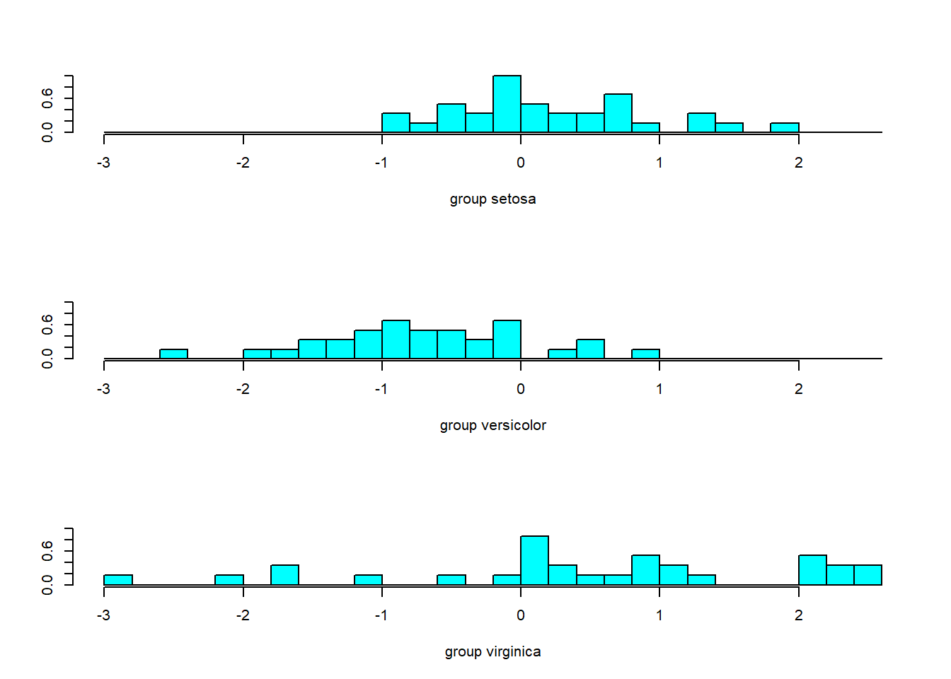

As we can see from the histogram here above LD2 we have a lot of overlap, which is not great. Now we can try to create the Bi-Plot.

# # Bi-Plot
library(ggord)
ggord(linear, training$Species, ylim = c(-10, 10))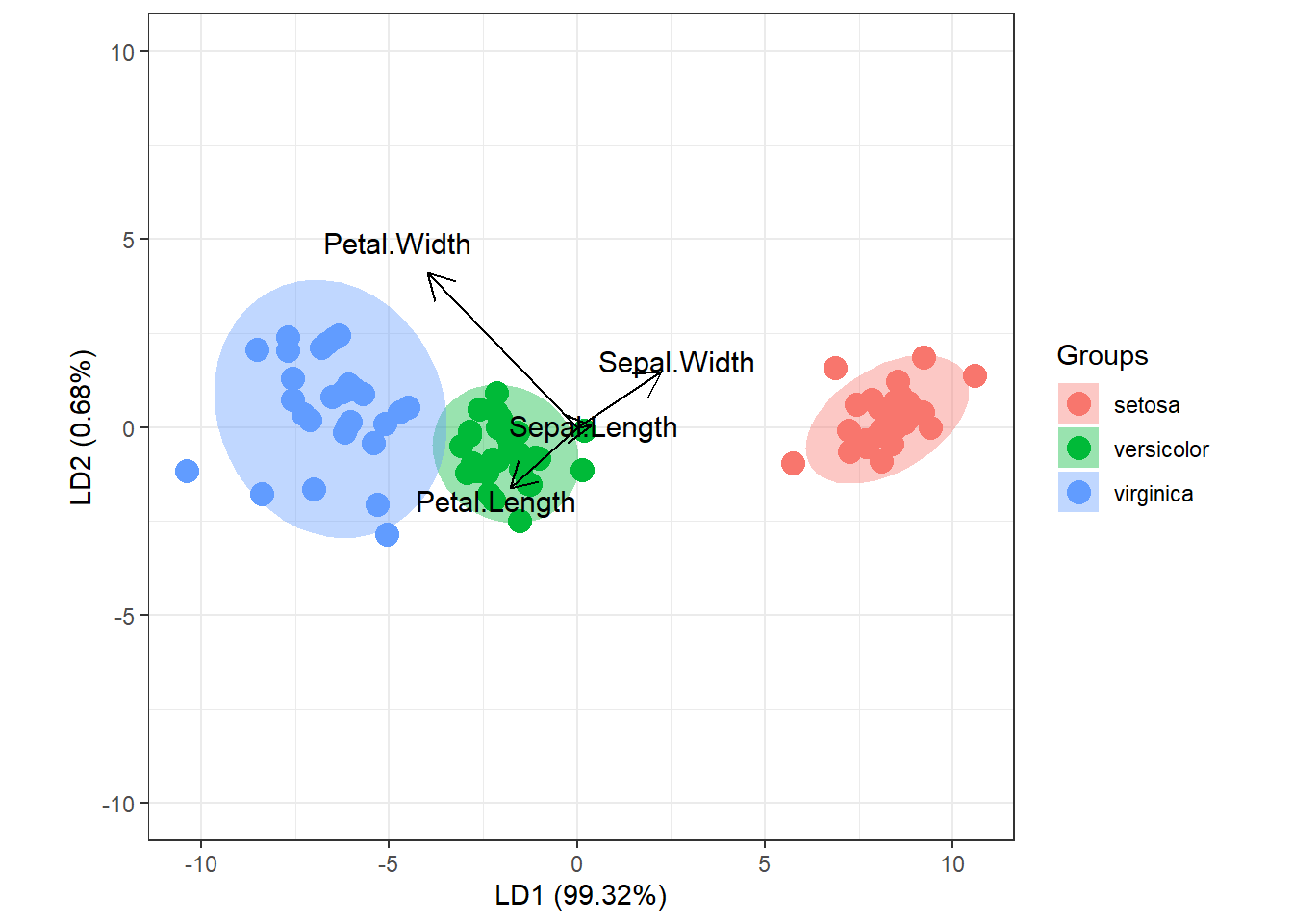

From the Bi-Plot above, we have in the x-axis the LD1 and is able to separate the three Species quite well. There is some amount of overlap between versicolor in green and virginica in blue. We can also see that Sepal.Width and Sepal.Length are both in a positive direction. The contrary is for Petal.Width and Petal.Length.

Now we can build the Partition Plot.

# # Bi-Plot with Linear Discriminant Analysis Model
library(klaR)
partimat(Species~., data=training, method="lda")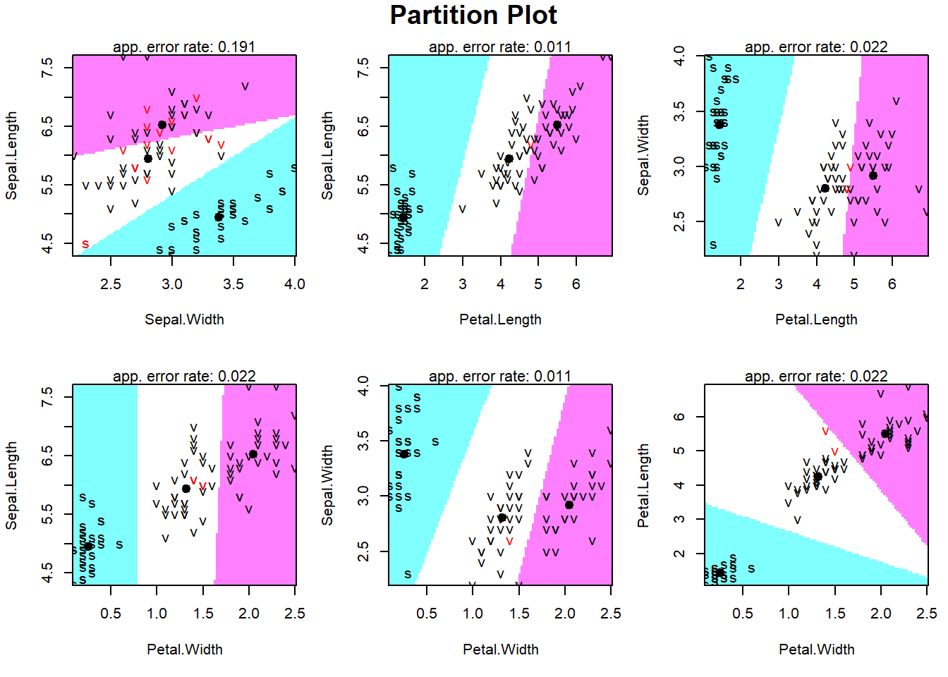

From the Partition Plot above, we can see classification for eachof observation in the training dataset based on the Linear Discriminant Analysis Model, and for every combination of two variables. From the right bottom graph, we can see that setosa s is quite far away from the other two Species, and bewtween versicolor and virginica there is some amount of overlap. The graph above is for a Linear Discriminant, we can also use a Quadratic Discriminant Analysis Model.

# Bi-Plot with Quadratic Discriminant Analysis Model
partimat(Species~., data=training, method="qda")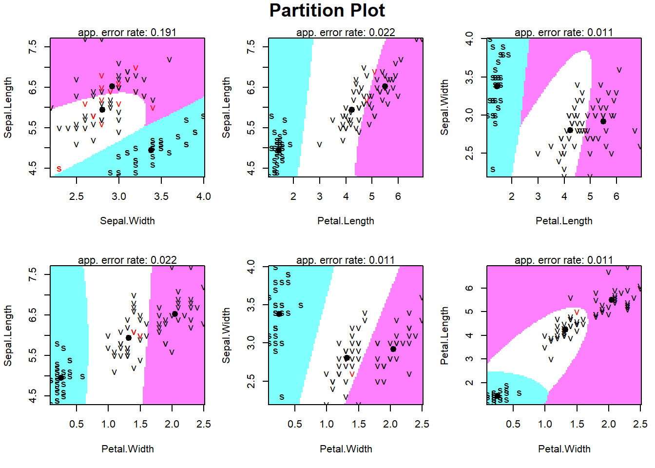

# Confusion Matrix and Accuracy
p1 <- predict(linear, testing)$class
tab1 <- table(Predicted = p1, Actual = testing$Species)
tab1

            Actual
Predicted    setosa versicolor virginica
  setosa         20          0         0
  versicolor      0         19         1
  virginica       0          1        20

accuracy1 <- sum(diag(tab1))/sum(tab1)
accuracy1

[1] 0.9672131

# Quadratic Discriminant Analysis
quadratic <- qda(Species~., data=training)

p2 <- predict(quadratic, testing)$class
tab2 <- table(Predicted = p2, Actual = testing$Species)
tab2

            Actual
Predicted    setosa versicolor virginica
  setosa         20          0         0
  versicolor      0         16         2
  virginica       0          4        19

accuracy2 <- sum(diag(tab2))/sum(tab2)
accuracy2

[1] 0.9016393

From the Partition Plot above, now we have a curve to discriminate between Species. From the Accuracy estimation of the testing data, we can see that is higher with Linear Discriminant Analysis Model (96.72% vs. 90.16%), which is also confirmed comparing the confusion matrix for the linear discriminat (tab1) vs. the confusion matrix of the quadratic discriminant (tab2).