Generalized Addictive Models GAMs incorporates non linear form of predictions, and are useful when we have not linearity between response variable and predictors. GAMs doesn’t force the predictors to a square as in polynomial regression, but GAMes tries to do a smooth line. The data we use here is biocapacity of different countries.
library(psych)
eco <- read.csv("C:/07 - R Website/dataset/ML/biocap.csv")

pairs.panels(eco,
             method = "pearson", # correlation method
             hist.col = "#00AFBB",
             density = TRUE,  # show density plots
             ellipses = FALSE # show correlation ellipses
             )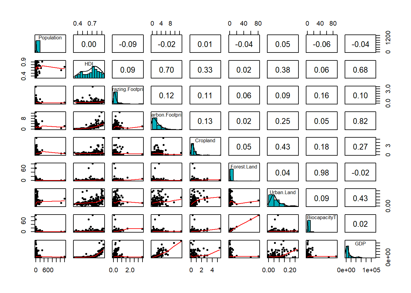
From the scatterplot above, we can see we have quite curve relationship between Human Development Index HDI and Gross domestic product GDP. Now we can try to build a Generalized Addictive Model with BiocapacityT as response variable.
library(mgcv)
# GAM model
mod_lm = gam(BiocapacityT ~ Population+HDI+Grazing.Footprint+Carbon.Footprint+
                Cropland+Forest.Land+Urban.Land+GDP, data=eco)

                summary(mod_lm)
Family: gaussian
Link function: identity

Formula:
BiocapacityT ~ Population + HDI + Grazing.Footprint + Carbon.Footprint +
    Cropland + Forest.Land + Urban.Land + GDP

Parametric coefficients:
                    Estimate Std. Error t value Pr(>|t|)
(Intercept)        5.356e-01  5.065e-01   1.058    0.292
Population        -3.230e-04  5.959e-04  -0.542    0.589
HDI               -8.647e-01  8.646e-01  -1.000    0.319
Grazing.Footprint  2.206e+00  2.535e-01   8.703 4.82e-15 ***
Carbon.Footprint   1.611e-02  9.163e-02   0.176    0.861
Cropland           1.764e+00  1.496e-01  11.797  < 2e-16 ***
Forest.Land        1.098e+00  1.105e-02  99.364  < 2e-16 ***
Urban.Land        -2.958e+00  1.977e+00  -1.496    0.137
GDP                6.233e-06  8.969e-06   0.695    0.488
---
Signif. codes:  0 '***' 0.001 '**' 0.01 '*' 0.05 '.' 0.1 ' ' 1


R-sq.(adj) =  0.985   Deviance explained = 98.6%
GCV = 1.3504  Scale est. = 1.2754    n = 162
# concurvity(mod_lm)From the summary results above, we can see tht GDP is not statistically significant. one aspect with GAMs is the Concurvity. It refers to the generalization of collinearity to the GAM setting. In this case it refers to the situation where a smooth term can be approximated by some combination of the others. Can lead to unstable estimates. If fact, Concurvity can be viewed as a generalization of co-linearity, and causes similar problems of interpretation. We have to drop one of the variable with concurvity.
# Instead of splines specify tensor product smooth
mod_gam3 <- gam(BiocapacityT ~ te(Grazing.Footprint, Cropland, Forest.Land), data=eco)
concurvity(mod_gam3)
para te(Grazing.Footprint,Cropland,Forest.Land)
worst 2.123046e-16 8.161468e-15
observed 2.123046e-16 3.681739e-33
estimate 2.123046e-16 8.832898e-34vis.gam(mod_gam3, type='response', plot.type='persp',
phi=30, theta=30,n.grid=500, border=NA)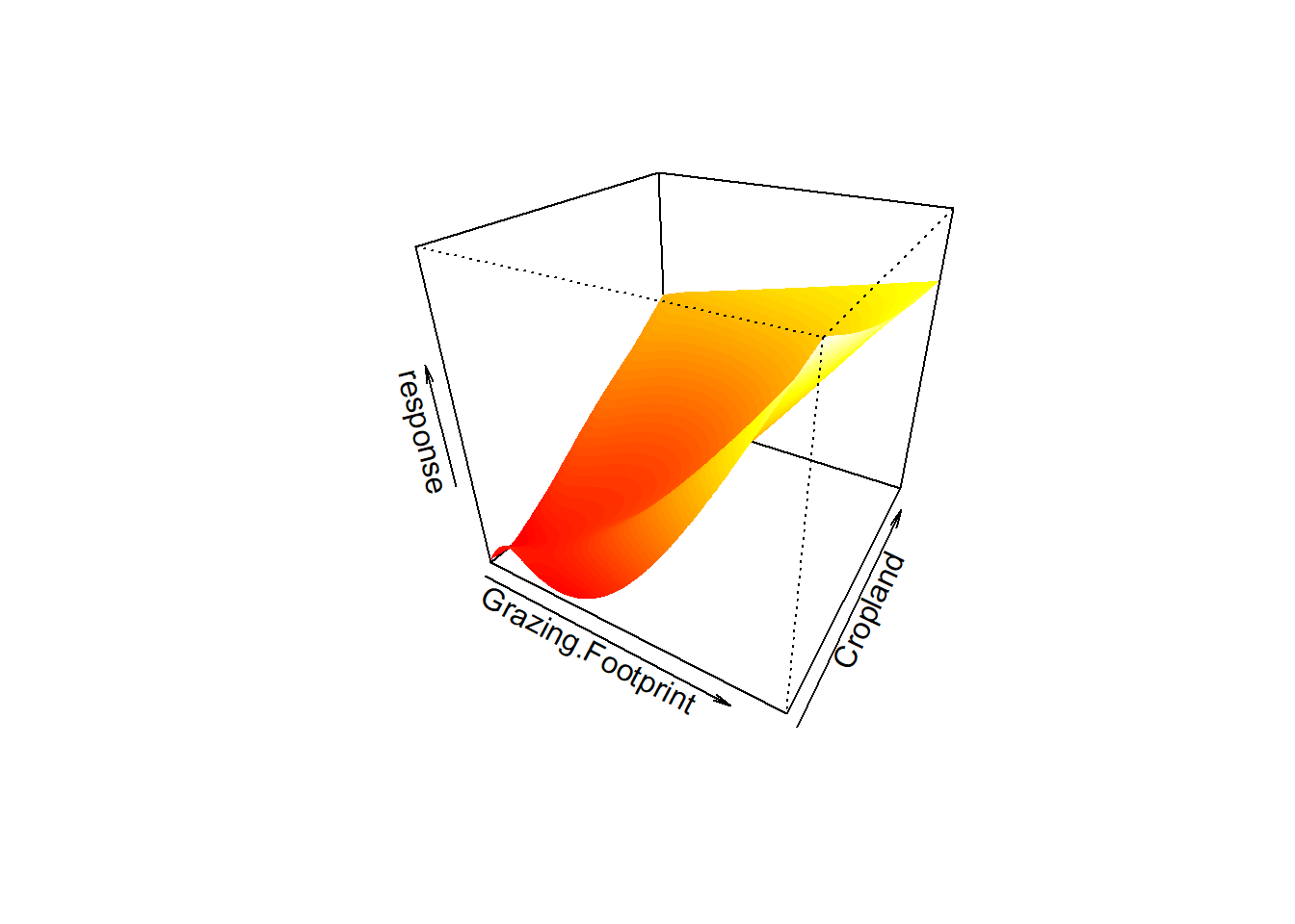 The model mod_gam3 uses the tensor smooth for predictors. If we look at the concurvity, in the worst case scenario Grazing.Footprint and Forest.Land have a strog relationship, but looking at the observed estimation the correlation is not very strong. The 3D visualization there is aportion that has come down (in red), and we can conclude for some extend that the predictors not contribute to the biocapacoty, and so we have to look to our data into more details.
Now, we try to use the R library caret() to tune parameters. By default it uses the smooth spline to mdel the relationship between response variable and independent variables. We use Leave One Out cross validation for the trainin set. We also use GCV as smoothing parameter.
# Instead of splines specify tensor product smooth
library(caret)

b = train(BiocapacityT ~ .,
           data = eco,
           method = "gam",
           trControl = trainControl(method = "LOOCV", number = 1, repeats = 1), # use leave one out cross validation
           tuneGrid = data.frame(method = "GCV.Cp", select = FALSE))


summary(b$finalModel)
Family: gaussian
Link function: identity

Formula:
.outcome ~ s(Urban.Land) + s(HDI) + s(Grazing.Footprint) + s(Cropland) +
    s(Forest.Land) + s(Carbon.Footprint) + s(Population) + s(GDP)

Parametric coefficients:
            Estimate Std. Error t value Pr(>|t|)
(Intercept)  3.61185    0.06785   53.23   <2e-16 ***
---
Signif. codes:  0 '***' 0.001 '**' 0.01 '*' 0.05 '.' 0.1 ' ' 1

Approximate significance of smooth terms:
                       edf Ref.df        F p-value
s(Urban.Land)        1.000  1.000    0.000   1.000
s(HDI)               1.598  1.993    1.164   0.320
s(Grazing.Footprint) 8.306  8.827   16.729  <2e-16 ***
s(Cropland)          3.270  3.934   59.088  <2e-16 ***
s(Forest.Land)       4.457  4.997 3271.685  <2e-16 ***
s(Carbon.Footprint)  1.000  1.000    0.036   0.850
s(Population)        1.479  1.768    0.421   0.524
s(GDP)               2.104  2.583    1.044   0.336
---
Signif. codes:  0 '***' 0.001 '**' 0.01 '*' 0.05 '.' 0.1 ' ' 1

R-sq.(adj) =  0.991   Deviance explained = 99.2%
GCV = 0.87676  Scale est. = 0.74572   n = 162
From the resut above wefound the most significant predictors, and we reached an Adjusted R-squared of 99% as before. We can now, use again the library caret() to deal with Concurvity and Collinearity.
About the smoothing parameter GCV we can say that both REML and GCV try to do the same thing. It has been shown that GCV will select optimal smoothing parameters (in the sense of low prediction error) when the sample size is infinite. At smaller (finite) sample sizes GCV can develop multiple minima making optimisation difficult and therefore tends to give more variable estimates of the smoothing parameter. If GCV is prone to undersmoothing at finite sample sizes, then we will end up fitting models that are more wiggly than we want, thought it best to switch to REML by default to avoid potential overfitting and highly variable smoothing parameter estimates.