Learning means to generalize what we learned and improve the performance of the same task based on a given measure. More specifically, it means to adjusting the parameters of the model in order to accurately predict the dependent variables on new input data. More formally we can define two main functions: the Score Function and the Loss Function. The score Function describes our mapping from the input space x to the output space y. The Loss Function measures the quality of a particular set of parameters based on how well induced scores agreed with the ground truth labels in the training set. The ultimate goal is to minimize the Loss Function. An example of loss function for the regression problem could be the classical mean squared error loss:
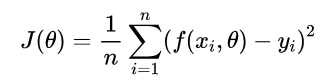
For each data points in our tuning set, we take the squared difference between the actual label yi and the output of the score function. Than, we normalize their sum by the total number of observations N. Other common Loss Functions are the Cross-Entropy Loss Function and the Hinge Loss Function. In the first case the output of the network are interpreted as log probability and in Hinge Loss Function we try to maximize directly the margin between the two classes. A very important note is to always remember to add the Regularization Term in the Loss Function formalized as follow:
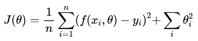
Here above, an eample using the L2 Regularization. We just need to add to the Loss Function designed before the regularization term. This help us to prevent overfitting.
Optimization Algorithms and Stochastic Gradient Descent Mathematical optimization is the selection of a best elements from some set of available alternatives. More formally, given a function f, we want to find an element such as f is minor or equal to f(x) for all the x in A, where A is a set of real numbers. An optimization process could be exact or approximate, which means it cannot guarantee to find the optimal solution. In the context of Deep Learning, having to deal with large number of parameters, and an unknown Loss Function Surface, an approximate algorithm is generaly prefered.
The easiest way to minimize a function is the so called Random Selection: we can just try all the possible combination of values in the domain of parameters and choose the set that corresponds to the minimum value of the loss function. In the real world we don’t have unlimited resources to perform the Random Search approach. The solution is to chose the parameters randomly. We can repeat this operation as many times we want and just keep track of the set of parameters that minimize the loss function. Random Search is never used in practice, especially if the parameter space is very large like in Deep Learning models.
A second approach is the Random Local Search, instead of trying many random sets of parameters, we can start with a Random Solution of Parameters and than Update such parameters with a random perturbation only if it leads to better solution. With this method we do not start from scratch at each iteration but we try to improve the current solution. Even though Random Local Search is better than Random Search, it is still wastefull and computationally expensive.
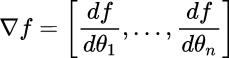
For this reason the Gradient of a function is used. In one-dimentional function, the derivative (slope) is the instantaneous rate of change of the function at any point we might be interested. When the functions of interest is multi-dimentional, we call the derivatives Partial Derivatives, and the gradient is simply the vector of partial derivatives in each dimenision.
This approach is called Stochastic Gradient Descent, or Mini-Batch Gradient Descent. The Classical Gradient Descent is one big batch containing the entire training set.