When we have to deal with a classification with more than 2 possible levels, we use a generalization of the logistic regression function called softmax regression; a logistic regression class for multi-class classification tasks. In Softmax Regression, we replace the sigmoid logistic function by the so-called softmax function.
\[ \begin{array}{l}{\qquad P\left(y=j | z^{(i)}\right)=\phi_{\text {softmax}}\left(z^{(i)}\right)=\frac{e^{z^{(i)}}}{\sum_{j=0}^{k} e^{z_{k}^{(i)}}}} \\ {\text { where we define the net input } z \text { as }} \\ {\qquad z=w_{1} x_{1}+\ldots+w_{m} x_{m}+b=\sum_{l=1}^{m} w_{l} x_{l}+b=\mathbf{w}^{T} \mathbf{x}+b}\end{array} \]
The w is the weight vector, x is the feature vector of 1 training sample, and b is the bias unit. A bias unit is an extra neuron added to each pre-output layer that stores the value of 1. Bias units aren’t connected to any previous layer and in this sense don’t represent a true activity. It is used in the case the sum of the weights is equal to zero. Now, this softmax function computes the probability that this training sample x(i) belongs to class j given the weight and net input z(i). So, we compute the probability p(y=j∣x(i);wj) for each class label in j=1,…,k.. Note the normalization term in the denominator which causes these class probabilities to sum up to one.
Even if it is a bit unusual, we use the softmax regression as the activation function of the output layer y.
\[ \begin{array}{l}{t=e^{\left(z^{(1)}\right)}} \\ {a^{(L)}=\frac{e^{z^{(L)}}}{\sum_{j={1}}^{4} t_{i}}, \quad a_{i}^{(L)}=\frac{t_{i}}{\sum_{j={1}}^{\frac{4} t_{i}}}}\end{array} \] The formula above assumes that we have 4 layers L on the output y as depicted in the figure below.
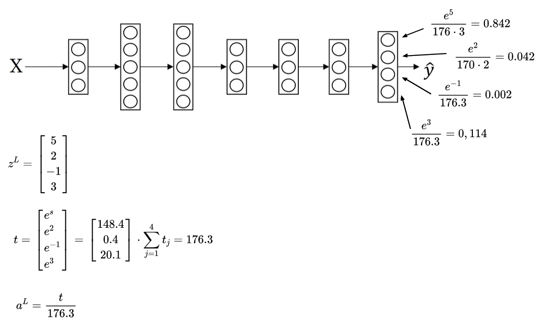
In the figure above we have z^(L) set to (5, 2, -1, 3), and from these values we can compute the activation function t suing the formula represented in the calculation we made before. Having the value of t, we can calculate the activation function a for the output y. From the example above, the output with level_0=0.842 is the most likely to categorize what we received in input. The categorization is called hard max and gives 1 to level_0 and 0 to the other output values. On the contray, the value 0.842 is called soft max.
The loss function L is calculated as follow: \[ f(\hat{y}, y)=-\sum_{j=1}^{4} y_{j} \log \hat{y}_{j} \]
For the values categorized with 0 in hard max, the yi is zero and so the loss finction is just equal to -log(yi). More generally, what the loss function does is to looks, at whatever is the ground true in our training-set, at the correspoding probability of that class and put it as high as possible. This is quite similar to the maximum likehood estimation.
Reference: coursera deep neural network course