RNN is a Supervised Deep Learning used for Time Series Analysis. Recurrent Neural Networks represent one of the most advanced algorithms that exist in the world of supervised deep learning.
Frontal lobe and RNN RNNs are like short-term memory. We will learn that they can remember things that just happen in a previous couple of observations and apply that knowledge in the going forward. For humans, short-term memory is one of the functions of the Frontal Lobe.
The idea behind RNN The idea is that weights have Long Term Memory abbreviated as LTM. For example, in a classical ANN known the weights, and so whatever input, we put into the ANN, it will process it in the same way as it would yesterday. The weights can be located in the Temporal Lobe of a human brain, because the Temporal Lobe is responsible for Long Term Memory LTM. RNN is like Short Term Memory, because it can remember things that are just happened in the previous couple of observations. The figure below is a representation of RNN.
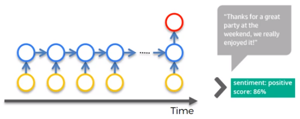
The circle in blue, that represent the hidden layer, is called the Temporal Loop,and they are connected through time. It is a sort of short term memory, able to remember what was in that neuron just previously. For example, when we have a lot of text, we need to gauge if it is a negative or a positive comment this RNN is called Many to One. Another example is Google Translator which is a very sophisticated deep learning. For example it is able to adapt the translation based on the gender. For example in english we can say: I am a boy/girl and I love to read. But the translation in Italian for a boy is: Sono un ragazzo e amo leggere. The translation for a girl is instead: Sono una ragazza e amo leggere. This RNN is called Many to Many. The concept here is that we need the memory of the content in order to solve this translation problem.
Vanishing Gradient In the gradient descent we have to find the global minimum in order to have an optimal solution. In RNN when the information is traveling through the network there are lots of error to evaluate, and we have to remember that the blue nodes are not just neurons but a complete hidden layer. Now, every single neuron which participate in the calculation of the output should have its weight updated in order to minimize the error. The Weight Recurring Wrec in temporal loop have to be updated many times and they become small. Now, the point is that when we multiply the weights, our value decreases very quickly, and Wrec become smaller.
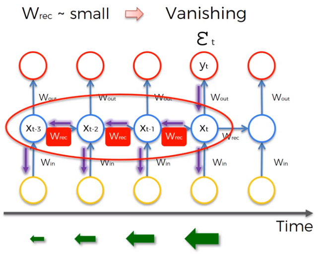
As described by the green arrows at the bottom of the figure, when the gradient goes back through the network the lower the gradient is. The consequence is that the lower the gradient and the slower is the process to update the weights like a domino effect. The solution is the Long short-Term Memory Network LSTMs.
Long short-Term Memory Network LSTMs The faster solution to solve Vanishing Gradient is to give a value to the Weight Recurring Wrec a value less than one: Wrec < 1 or Wrec = 1.
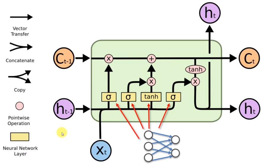
The C stand for Memory of the Cell. The h is the output, and the X is the input. Any black line in the schema is a vector. The operators are the x or valve and like in plumbing we can open or close it, and when the valve is open the memory goes freely, and the memory is controlled by the sigmoid function represented by the sigma symbol in the graph above. For example, opening a valve can help to extract the gender in Google Translator. In other words is the best solution to predict text. The + symbol stands for the T-Shape joint, and it is used to add some additional memory in the flow. The Hyperbolic Tangent Activation Function for short tanh operator goes between -1 and 1, allowing for increases and decreases in the state. There are also some variations of the LSTM, for example the so called Gated Recurring Unit or GRUs for short. Here, the C memory cell is completely ignored, and it is replaced by the output h.
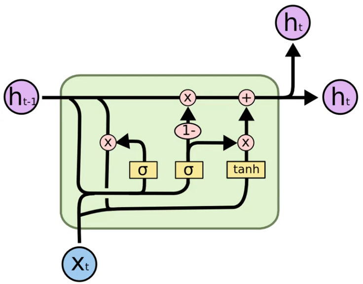
Here the new hidden state in the previous hidden state is combined to form a vector. Than is goes through the tanh activation function Hyperbolic Tangent Activation Function. That helps to regulate flowing through the network, and it ensures that values remain between -1 and 1. Thanks to the tanh all the information are maintained, instead using the Sigmoid activation Function we can lose information because small values go close to zero and so they disappear.
In short, Gated Recurrent Units GRUs have what is called an update gate and a reset gate. Using these two vectors, the model refines outputs by controlling the flow of information through the model. Gates are expressed by the Sigmoid Function: 0 = do not update weight, 1 = update weight.