Having a one layer neural network (single layer feedforeward) with the output value to be compare to the actual value. Baed on the activation function we have our output. In order to be able to lear, we have to compare the output value with the actual value via the cost funtion which is the half of the squred difference output and actual value. Cost function says that is the error in our prediction: the lower the cost function the closer the output value to output value. So, the information is going back and our weights have been updated till we minimize the cost function. This process is called back propagation.
Batch Gradien Descent How can we minimize the cost function? The figure represent our cost function and represent the best way to find the best soution for our weights. We continue to calcuate the slope in the points represented by the red dot till we find the best weights, the best situation that minimize the cost function. This process is also know as batch gradient descent because evaluete all observations at once.
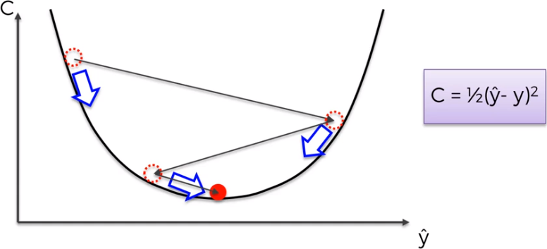
The problem is that this method requires for the cost function to be convex. If our function is not convex like in a multidimentional space, we could find a local minimum rather than the global one and we are not able to optimize our neural network.
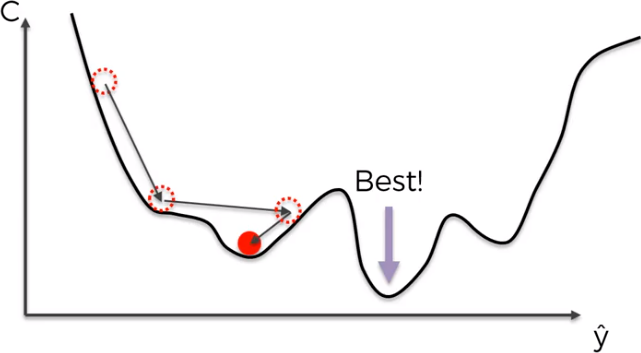
The solution is the Stocastic Gradient Descent that doesn’t require the cost function to be convex. Here, we take each observation one by one and we adjust the weights. It is not like the batch gradient descent where we use all observations at once. This approach avoid the problem local minimums.
Backpropagation This method allows to adjust weights all at the same time. The huge advantage is that during the process of back propagatins we are able to adjust all the weights at the same time and so we know which part of the error each of our weights in the network is responsable for. STEP 1: randomly initialise the weights to close to zero (but not 0). STEP 2: forward propagation: from left to right, the neurons are activated in a way that the impact of each neuron’sactivation is limited by the weights. Propagate the activations until getting the predicted result y. STEP 3: compare the predicted result to the actual result. Measure the generated error. STEP 4: back propagation: from right to left, the error is back propagated. update the weights according to how much they are responsible for the error. STEP 5: repeat STEP 1 to 4 and update the weights after each observation (Reinforcement Learning). Or, repeat STEP 1 to STEP 4 but update the weights only after a batch of observation (Batch Learning).
Reinforcement Learning exampe: Predict the exit of the costomers of a bank
The dataset contain information about the customers in a bank and if thy stay or left the bank within a six month period (Exited). Our goal is to predict the exited from all the feuture that we have about each customer.
| CreditScore | Geography | Gender | Age | Tenure | Balance | NumOfProducts | HasCrCard | IsActiveMember | EstimatedSalary | Exited |
|---|---|---|---|---|---|---|---|---|---|---|
| 619 | France | Female | 42 | 2 | 0.00 | 1 | 1 | 1 | 101348.88 | 1 |
| 608 | Spain | Female | 41 | 1 | 83807.86 | 1 | 0 | 1 | 112542.58 | 0 |
| 502 | France | Female | 42 | 8 | 159660.80 | 3 | 1 | 0 | 113931.57 | 1 |
| 699 | France | Female | 39 | 1 | 0.00 | 2 | 0 | 0 | 93826.63 | 0 |
| 850 | Spain | Female | 43 | 2 | 125510.82 | 1 | 1 | 1 | 79084.10 | 0 |
| 645 | Spain | Male | 44 | 8 | 113755.78 | 2 | 1 | 0 | 149756.71 | 1 |
| 822 | France | Male | 50 | 7 | 0.00 | 2 | 1 | 1 | 10062.80 | 0 |
| 376 | Germany | Female | 29 | 4 | 115046.74 | 4 | 1 | 0 | 119346.88 | 1 |
The first step is to encode the categorical variables as factors.
dataset$Geography = as.numeric(factor(dataset$Geography,
                                      levels = c('France', 'Spain', 'Germany'),
                                      labels = c(1, 2, 3)))

dataset$Gender = as.numeric(factor(dataset$Gender,
                                   levels = c('No', 'Yes'),
                                   labels = c(0, 1)))
Now, we split the data into Training and Test Set.
library(caTools)
set.seed(123)
split = sample.split(dataset$Exited, SplitRatio = 0.8)
training_set = subset(dataset, split == TRUE)
test_set = subset(dataset, split == FALSE)
We are going to the final step of data pre-processing and it is Feature Scaling. We need to apply feature scaling to train the Artificial Neural Network.
training_set[-11] = scale(training_set[-11])
test_set[-11] = scale(test_set[-11])
Now is time for action and build our ANN. There are several deep learning packages in R, but probably the best is H2O because is an oper source software platform that allows us to connect to an instance of a computer system that therefore allows us to run our model very efficiently. It like in Python when you connected to GPU that allows you to run highly computer intensive parallel computation. Moreover, H2O offers a lot of options to use different number of hidden layers. It is also very important to note that H2O contains a Parameter Tuning argument that allows us to choose some optimal number to build the deep learning model.
library(h2o)
h2o.init(nthreads = -1)
Connection successful!
R is connected to the H2O cluster:
H2O cluster uptime: 2 hours 57 minutes
H2O cluster timezone: Europe/Berlin
H2O data parsing timezone: UTC
H2O cluster version: 3.20.0.8
H2O cluster version age: 3 months and 24 days !!!
H2O cluster name: H2O_started_from_R_perlatoa_hkx874
H2O cluster total nodes: 1
H2O cluster total memory: 2.48 GB
H2O cluster total cores: 4
H2O cluster allowed cores: 4
H2O cluster healthy: TRUE
H2O Connection ip: localhost
H2O Connection port: 54321
H2O Connection proxy: NA
H2O Internal Security: FALSE
H2O API Extensions: AutoML, Algos, Core V3, Core V4
R Version: R version 3.5.1 (2018-07-02) model = h2o.deeplearning(y = 'Exited',
training_frame = as.h2o(training_set),
activation = 'Rectifier',
hidden = c(5,5),
epochs = 100,
train_samples_per_iteration = -2)
  |
  |                                                                 |   0%
  |
  |=================================================================| 100%

  |
  |                                                                 |   0%
  |
  |=================================================================| 100%
Now, we can predict the Test results.
y_pred = h2o.predict(model, newdata = as.h2o(test_set[-11]))
  |
  |                                                                 |   0%
  |
  |=================================================================| 100%

  |
  |                                                                 |   0%
  |
  |=================================================================| 100%
y_pred = (y_pred > 0.5)
y_pred = as.vector(y_pred)And making the Confusion Matrix.
cm = table(test_set[, 11], y_pred)
cm
y_pred
0 1
0 1537 56
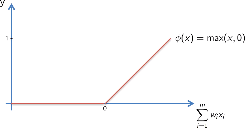
1 219 188As you can see from the code above we use the Rectifier Function as activation function (best option). See here below a quick emind of the rectifier function. Based on experiments, a convenient choice of number of hidden neurons is the average of the number of input features plus the number of output y. The prameter train_samples_per_iteration = -2 says to auto-tuning the model.
A quick refresher about Activation Function.
We have four different types of activation functions that we can choose from. Threshold function, Sigmoind function, Hyperbolic Tangent. But the Rectifier function is the most popular function for Artificial Neural Network. It goes all the way to zero, and from there it gradually progresses as the input value increases as well.
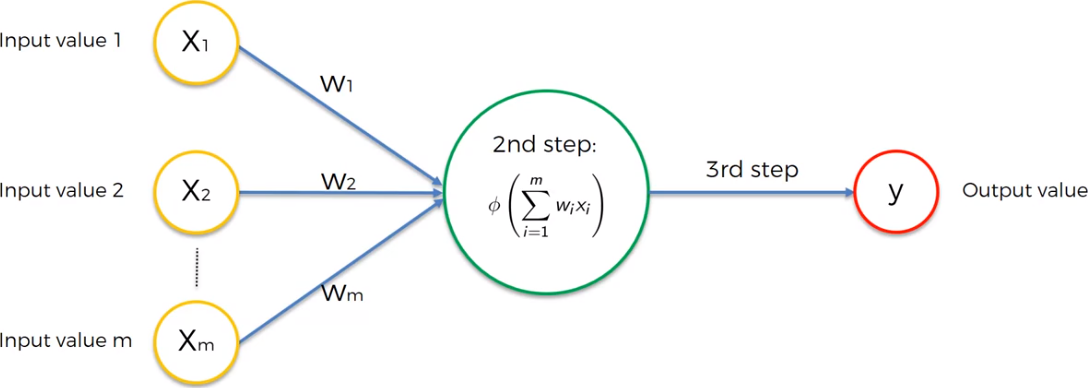
The neuron representation above reflect the problem that we are facing. In fact, we have just a binary output and m number of feature as input. It such a context, we can choose one of the four activation functions mentioned above. But, that what should be used for a binary problem? There are two options: 1 - Rectifier function for the hidden layer 2 - Sigmoid function for the output layer.