Introduction We already know that there is in ANN a Forwward Propagation where the information is entered into the input layer, and then it is propagated forward to get our output values to compare with the actual values that we have in our training set, and then we calculate the errors. Then the errors are back propagated through the network in the opposite direction in order to adjust the weights. An importan thing to remember is that Back Propagation is an advanced algorithm which allows us to adjust the weights all of them at the same time. We are able to know which weight is responsable for the error.
The basic idea of backpropagation is to guess what the hidden units should look like based on what the input looks like and what the output should look like. The definition of backpropagation is a way of computing gradients through recursive application of chain rules. It is the standard way of computing gradients for ANNs. It is a very flexible solution for comupting the gradient through simple, incremental steps. The first step is to understand what the Chain Rule is all about.
Chain Rule The fundamental unit of every deep learning model is the Perceptron. The Perceptron algorithm was designed to classify visual inputs, categorizing subjects into one of two types and separating groups with a line: it is used for linearly-solvable problems.
In calculus, the Chain rule is a formula for computing the derivative of the composition of two or more functions called Perceptron. The Chain Rule allow us to break down a complex function in many smaller functions for which it is relatively straighforward to compute the derivative. Then, we simply chain them together by multiplication.
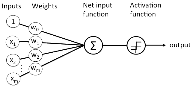
Let’s assume we have a set of neurons with weght as described by the figure below.
We can apply an Activation Function in order to have a smoother ranging from 0 to 1, for example the Sigmoid Function described by the formula below.
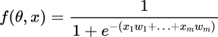
We want to compute the derivative with respect of the weight w0 till to wn. First of all, we semplify the function introducing the g tems.
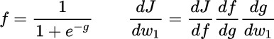
Once we have the Gradient of the Loss Function with respect to All the Weights we can update our model simply by the function below, that make a subtraction of the gradient by alfa times which is the the learinign rate. Here, for semplicity, is not consider the Regularization term, but we have to remember to always take it into consideration, especially for large models. Of course, we don’t have to go through all this math each time we want to develop a new deep learning model, but we can use the fully-fledged packages.
Hyper-parameters Optimization Tillnow, we have seen how to Learn the Weights of the Perceptron on any Deep Learning Models. There are possibility to automatic tuning the hyper-parameters especially using Random Search and Grid Search.
In the following example, we consider to tuning the hyper-parameter using the Stochastic Gradient Descent. In general, evaluating the Loss Function with respect to the hyper-parameters means training the model from scratch each time which makes the problem computationally impossible to solve. That is why, it is pretty common to tune the hyper-parameters manually with some tricks such as Grid Search, Random Search, and Bayesian Methods.
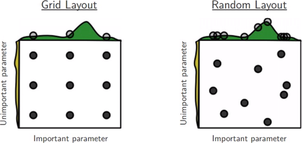
Let’s say we want to tune just two hyper-parameters, and each of the boxes represented by the figure above, represent the hyper-parameter space in which we can choose the hyper-parameter. Since we can not test each possible combinations of th two hyper-parameters we can decide to cover the space with Discrete values in Grid Search, and Random Pairs in Random Search. It turns out that in general the Random Layout is better than the Grid Layout because for the hyper-parameters we can test more different values for the Important Parameters. More pratically, we can implement a Random Search in R using H2O which come with a complete set of utility functions specifically designed for this purpose. The h2o.grid() function is very general and adapttive an helps to implement the Grid or Random Search with few lines of R code even for a comple hyper-parameters selection.
In the following example we use the Wisconsin Breast-Cancer Dataset which is a collectioin of Dr.Wolberg real clinical cases. There are no images, but we can recognize malignal tumor based on 10 biomedical attributes. We have a total number of 699 patients divided in two classes: malignal and benign cancer.
# Load libraries
library(mlbench)
library(h2o)

# General parameters
h2o.init()
H2O is not running yet, starting it now...

Note:  In case of errors look at the following log files:
    C:\Users\perlatoa\AppData\Local\Temp\Rtmp0IbWAd/h2o_perlatoa_started_from_r.out
    C:\Users\perlatoa\AppData\Local\Temp\Rtmp0IbWAd/h2o_perlatoa_started_from_r.err


Starting H2O JVM and connecting: . Connection successful!

R is connected to the H2O cluster:
    H2O cluster uptime:         4 seconds 620 milliseconds
    H2O cluster timezone:       Europe/Berlin
    H2O data parsing timezone:  UTC
    H2O cluster version:        3.20.0.8
    H2O cluster version age:    8 months and 30 days !!!
    H2O cluster name:           H2O_started_from_R_perlatoa_toc367
    H2O cluster total nodes:    1
    H2O cluster total memory:   2.65 GB
    H2O cluster total cores:    4
    H2O cluster allowed cores:  4
    H2O cluster healthy:        TRUE
    H2O Connection ip:          localhost
    H2O Connection port:        54321
    H2O Connection proxy:       NA
    H2O Internal Security:      FALSE
    H2O API Extensions:         AutoML, Algos, Core V3, Core V4
    R Version:                  R version 3.5.1 (2018-07-02)
set.seed(1)
# Load the data
data(BreastCancer)
# Convert data for h2o
data <- BreastCancer[, -1] # remove ID
data[, c(1:ncol(data))] <- sapply(data[, c(1:ncol(data))], as.numeric) # interpret each features as numeric
data[, 'Class'] <- as.factor(data[, 'Class']) # interpret dependent variable as factor
# convert the dataset in three part in the h2o format
splitSample <- sample(1:3, size=nrow(data), prob=c(0.7,0.15,0.15), replace=TRUE)
train_h2o <- as.h2o(data[splitSample==1,])
  |
  |                                                                 |   0%
  |
  |=================================================================| 100%
valid_h2o <- as.h2o(data[splitSample==2,])
  |
  |                                                                 |   0%
  |
  |=================================================================| 100%
test_h2o <- as.h2o(data[splitSample==3,])
  |
  |                                                                 |   0%
  |
  |=================================================================| 100%
Now, we can choose the best hyper-parameters using the Random Search. As we can see from the code below, we try to use many Activation Functions, many Hiden Layers with different units, different Drop-out Ratio, and L1 and L2 Regularization.
# Set hyper-parameters
hyper_params <- list(
  activation =c("Rectifier", "Tanh", "Maxout",
                "RectifierWithDropout", "TanhWithDropout", "MaxoutWithDropout"), # different activation function
                hidden = list(c(20,20), c(50,50), c(30,30,30), c(25,25,25,25)), # different layers with different units
                input_dropout_ratio = c(0, 0.05), # different drop-out ratio
                l1 = seq(0, 1e-4, 1e-6), # L1 regularization
                l2 = seq(0, 1e-4, 1e-6)) # L2 regularization
The Activation Functions used are: Rectifier, Tanh, Maxout, and we use different Drop-out Ration. The Drop-out process is about Pruning some connections between neurons during training. It is very attractive to know that the human brain do the same pruning process in the early stage of the birth.
Now, we need to define the search criteria, and in the following example we use the Random Search criteria.
# Set the search criteria
search_criteria <- list(
  strategy = "RandomDiscrete", max_runtime_secs = 360, # maximum time in seconds for the entire Random or Grid
  max_models = 100, seed=1234567, stopping_rounds = 5, # maximum time in seconds for he model
  stopping_tolerance = 1e-2 # the model will stop if the ratio between the best model and reference is more or equal to 1e-2
)
Now, we can use the h2o.grid() function to compute all the models defined. We specify deeplearning as the algorithm. We also defined to stop the training every single model when the logloss is not improved more than 1% after 2 different evaluations. In the end, we can guess the best model using the function h2o.getModel() and taking the first model, since the models are ordered.
About the Log-Loss function a simple explanation is the following: consider to have the Predicted Probability Distribution of a Supervised Classifier, and also the True Distributon. We can use the Cross Entropy to estimate the difference between the Predicted Distribution and the True Distribution: this is called the Cross Entropy Loss or the Log-Loss. If the predicted probability calculated from the Log-Loss is closed to 1, then the cost will be closed to the True Distribution.
About Epochs is deep learning an epoch is a hyperparameter which is defined before training a model. One epoch is when an entire dataset is passed both forward and backward through the neural network only once. Using all your batches once is 1 epoch. If you have 10 epochs it mean that you’re gonna use all your data 10 times (split in batches).
# Define Grid
# dl_random_grid <- h2o.grid(
#   algorithm = "deeplearning", # use artificial neural network with unlimited number of hidden layers
#   grid_id = "dl_grid_random", # use Random Search
#   training_frame = train_h2o,
#   validation_frame = valid_h2o,
#   x = 1:9, # predictors
#   y =  10, # dependent variable
#   epochs = 1, # all bathces once
#   # stop when logloss does not improve by more than 1% after 2 evaluation
#   stopping_metric = "logloss", # cross entropy
#   stopping_tolerance = 1e-2,
#   stopping_rounds = 2,
#   hyper_params = hyper_params,
#   search_criteria = search_criteria # random search
# )
#
#
# # Recover the Grid
# grid <- h2o.getGrid("dl_grid_random", sort_by="logloss",
#                     decreasing = FALSE)
#
# grid@summary_table[1,]
#
# # Take the best model with lowest logloss
# best_model <- h2o.getModel(grid@model_ids[[1]])
# best_model
Using Grid and Random Search we can find out our model automatically maximazing the accuracy on the validation set.
Evaluate the Artificial Neural Network In order to understand how the model behaves after the REAL DEPLOYMENT we should: Split the data-set in 3 parts: Train (40%), Validation (30%) and Test (30%) set. In our exapme we used 70 for Train, 15 for Validation, and 15 for Test. We also need a Validation set because if we tune the hyper-parameters based on the results on the TEST set, we end-up overfitting it as well. Validation Sets are also known as Dev Sets, it is an intermediate phase used for choosing the best model and optimizing it. It is the parameter tuning that occurs for optimizing the selected model. Overfitting is checked and avoided in the validation set to eliminate errors that can be caused for future predictions if an analysis corresponds too precisely to a specific dataset. It is generally considered unwise to attempt further adjustment in the testing phase. Attempting to add further optimization outside the validation phase will likely increase overfitting.
Optimization Loss It helps to understand when Accuracy is saturating, for example, stop to add hidden layer in a Multi Hidden Layer ANN. Accuracy or Error, is what the model optimizes. There is a method called EARLY STOPPING: we stop the training when the model starts to work with the desired metric.

M1 error rate refer to the Training-set. M2 error rate refer to the Test-set. The point where M2 start to increase the error, means that the Neural Network stop to generalize. It stop understanding the pattern in the data. Crucially, after the Stopping point there is Overfitting. If we don’t receive our desired accuracy at the Stopping Point, we need to use a different NN, for example, changing the number of hidden layers.