The ultimate goal of survival analysis is to gain information on the expected duration of time untill one or even more events happen. Survival analysis is applied in different fields and most of these fields have different terms for the same concept. So, sometimes it is called Reliability Theory or Reliability Analysis in engineering. It is also called Duration Analysis in economics or Event-history Analysis is sociology. The underlying questions which the analysis tries to answer are as follows: 1 - What is the proportion of a population surviving past a certain time? 2 - Of those that survive, at what rate will they die or fail? 3 - Can multiple causes of death or failure be taken into account? 4 - What is the average survival time? 5 - How do particular circumstanses or characteristics change the probability of survival?
To answer these questions it is essential to define the Lifetime, the time before a certain event occured. essentially, the fundamental tools to describe the survival times of members of a group are Life Tables and Kaplan-Meier curves. To compare the survival times of two or more groups we mainly use the Log-rank test. To describe the effect of categorical or quantitative covariance on survival we mainly use the Cox Proportional Hazards Regression or Survival Tree and Survival Random Forest.
There are three primary terms of Survival Analysis: Event: depends on the study, e.g. failure, death, disease, recovery, decay, development. Usually is a binary event. Time: the time interval between the beginning of a study and the occurrence of the event. Censoring: occurs if a subject doesn’t have an event during the observational time. For example censoring happens when the subject no longer participates in the study without the event of interest taking place.
Prostate Cancer Dataset We will use as a template for survival analysis the prostate cancer dataset. The dataset come from a study on prosthetic cancer patients, and it contains several variables to indicate or are in correlation with prosthetic cancer. The data contain 63 patients and 8 independent variables. The main goal is to compare two different treatments identified with 1 or 2. Both ot these are surgical treatments which are pretty much indicative in higher stages of prostate cancer. The two tretments 1 and 2 differ in the amount of removed tissue and the type of tisue it was primarily removed. The time in the dataset was measured in months. The variable status can be 0=censoring (loss of follow up or quitting the study), or 1=no censoring. The variable sh is the blod measurement hormone. The variable size is the tumor size at the beginning of the study. The variable index is the Gleason Scoring System, because tumor has different stages and they actually start to metastasize other boby parts at higher index of Gleason Scoring System.
prost <- read.table("C:/07 - R Website/dataset/TS/prostate-cancer.txt", header = FALSE)

colnames(prost) = c("patient", "treatment", "time", "status", "age", "sh", "size", "index")
head(prost)
patient treatment time status age sh size index
1 1 1 65 0 67 13.4 34 8
2 2 2 61 0 60 14.6 4 10
3 3 2 60 0 77 15.6 3 8
4 4 1 58 0 64 16.2 6 9
5 5 2 51 0 65 14.1 21 9
6 6 1 51 0 61 13.5 8 8Non-parametric model The Kaplan-Meier estimation is often the first tool to use. It is mainly used as a step plot where an event indicates a decline in survival probability. The Survival Function, also called Reliability Function, gives the probability that a study subject will survive beyond a given specific time. Normally, the survival function has to be estimated, and the standard way to do this is via Kaplan-Meier estimator. The Kaplan-Meier plot, has on the x-axis the time passed and on the y-axis the sirviva probability. It is the statisticians way of estimating the survival function. The flat horizontal lines between the steps indicate an assumed constant survival function for that specific time period. A fairly important advantage of the Kaplan-Meier curve is the fact that this method can take into account censored data,and usually there censored data are indicated with a dot in the plot. On the other hand, an impostant limitation is the fact that we can not incorporate covariance into the estimate. This covariance would usually be handled with Cox Proportional Hazards Regression. What we often see is a chart comparing two or more Kaplan-Meier curves.
# Simply Kaplan-Meier plot
library(survival)
mykm1 <- survfit(Surv(time, status) ~ 1, data=prost)
mykm2 <- survfit(Surv(time, status) ~ treatment, data=prost) # group by treatment

library(ggfortify)
autoplot(mykm2)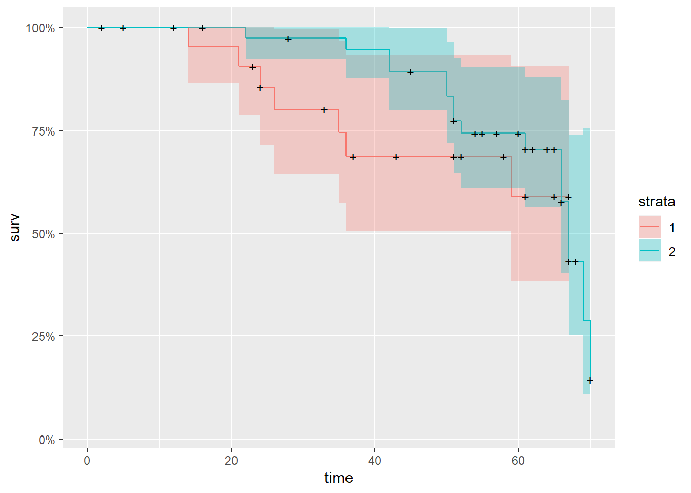
We can see the two Kaplan-Meier curves, one for the treatement 1 and the other for the treatment 2. Here, it is pretty obvious that treatment 2 has the better survival chances. For example at time 40 (40 months) the treatment 1 has already lower percentage of survival (around 70%), whereas treatment 2 is still at 95%. Now, after about 65 months the two curves are nearing each other and the probabilitis are equal. The censored data are reporesented witha little black cross.
The Logrank Test The Logrank Test is a fairly popular tool which allowsn two groups. In our case it helps to understand which treatment has a better survival probability. It is constructed by computing the obsrved and expected number of events in a group at each observed event time, and these numbers are then added up to get a total across all time points were there was an event. The Test statistics says that the Null Hypothesis is the hazard rate in each group is similar. The Null Hypothesis is rejected if the test statistic of Z is not normally distributed.
# Logrank Test
survival::survdiff(survival::Surv(prost$time, prost$status) ~ prost$treatment)
Call:
survival::survdiff(formula = survival::Surv(prost$time, prost$status) ~
prost$treatment)
N Observed Expected (O-E)^2/E (O-E)^2/V
prost$treatment=1 23 7 5.13 0.686 0.958
prost$treatment=2 40 16 17.87 0.197 0.958
Chisq= 1 on 1 degrees of freedom, p= 0.3 Looking at the reult of the Logrank Test here above, we can see the p-value which in this case is not significant, and so there is no difference in the survival probability of between the two treatments considered. From the result, we have also the total number of subjects per group N, as well as the expected events derived from the observed number. There is also the calculation of the chi-square statistics for each group, and the last column is the variance per group.