This article is a summary of the StatQuest video made by Josh Starmer. Click here to see the video explained by Josh Starmer.
The Principal Component Analysis is a deterministic method (given an input will always produce the same output). It is always good to perform a PCA: Principal Components Analysis (PCA) is a data reduction technique that transforms a larger number of correlated variables into a much smaller set of uncorrelated variables called Principal Components. For example, we might use PCA to transform many correlated (and possibly redundant) variables into a less number of uncorrelated variables that retain as much information from the original set of variables.
We can do that one step at a time using Singular Vector Decomposition. Imagine we are measuring the transcription of two genes: Gene1 and Gene2 that are our variables and six different mice, that are our observations. Or using another example: 6 types of businesses and the variables could be market capitalization and number of employees. Now, tha mice 1, 2, 3 have high value for Gene1 and mice 4, 5, 6 have low value for Gene2. So, mice 1, 2, 3 are more similar to each other than they are to mice 4, 5, 6.

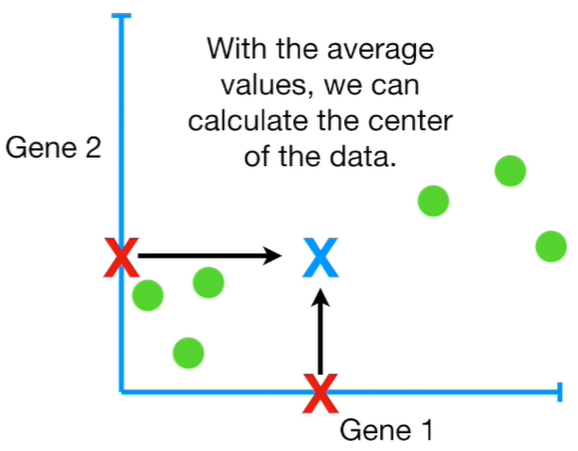
If we have more than 3 genes is quite difficult to use a four-dimensional graph to check where mice are allocated in that space. The Principal Component Analysis PCA, takes four or more-dimensional data and make a two-dimensional Principal Component Plot that is able to tell us which gene or variable is the most valuable for clustering the data. Now, let’s assume that we have only two genes and we just calculate two averages: one for gene1 and one for gene2. With this average we have now the Centre Average of the data, and we can shift the data so that the average is the origin of the graph.
Having the centre of data, allow us to start to draw a Random Line that goes through the origin that is the centre average. Then, we rotate the line until fits the data at best.
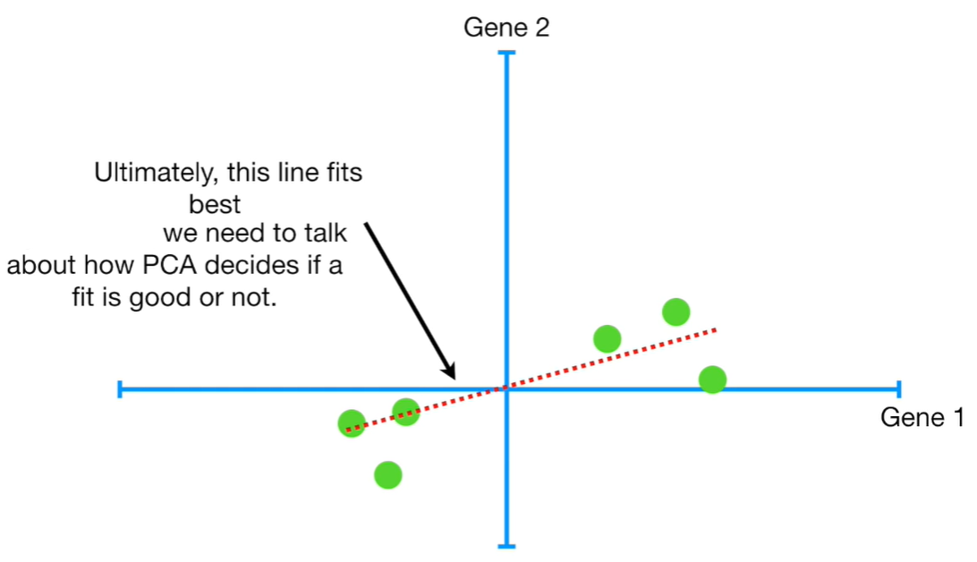
How to decide the line with best fit? The Principal Component Analysis simply projects the data onto the fitting line depiced above, and find the line that minimize those distances. And we can call D the distance between the projected points and the origin. The next step is to square all of them and we sum up the square distances: Sum of the Square Distances SS Distance. We repeat this procedure since we find the largest sum of square distances: this is called Principal Component One: which is also known as Linear combination between variables, in this example: gene1 and gene2.
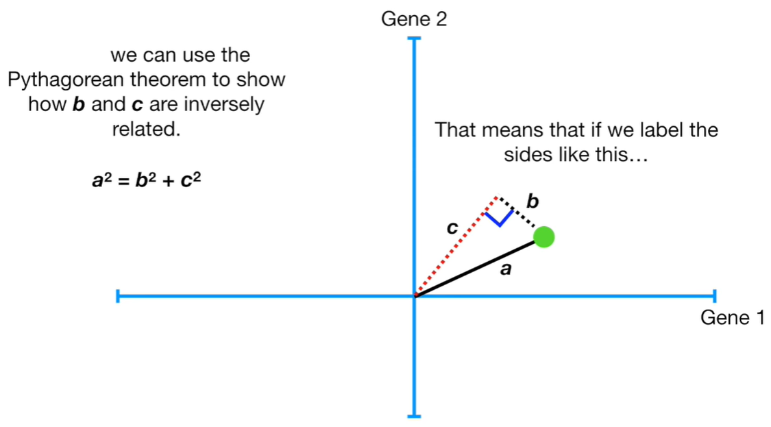
Now, from the distance on the x-axis and the distance from y-axis is possible to use the Pythagorean Theorem to find the hypotenuse of each observation and we scale it to a unit of one: this is called Singular Vector or Eigenvector for Principal Component One. This calculation that we make for all the observations is called Loading Scores. The square root of the eigenvector for PC1 is called the Singular Value for PC1.
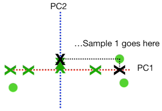
Now, let’s work on PC2: that is simple the line to the origin that is perpendicular to PC1, and from that line we can derive Eigenvector for PC2.
Now, we have an estimation for PC1 and PC2. To draw the final Principal Components graph, we simply rotate since PC1 is horizontal, and we use the projected points that we found to find where the observations go in the PCA graph (see graph below).
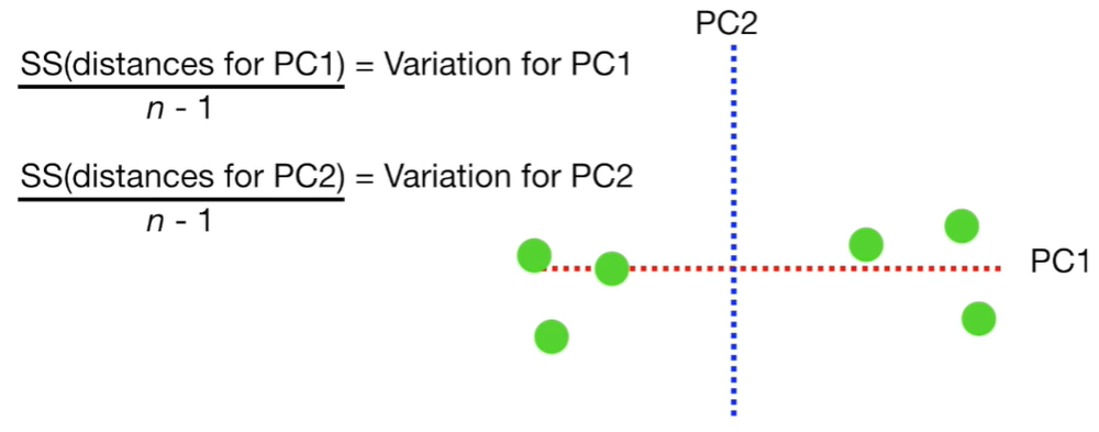
Now, if we divide eigenvalues for PC1 and eigenvalues for PC2 by the number of observations minus one, we obtain the Variation of PC1 and the Variation of PC2.
We now can use the so-called Screen Plot as a graphical representation of the percentages of variation that each Principal Components accounts for.
Note: if the first two Principal Components would not create a very accurate representation of the data, in this case could be better to use an Ensamble approach.
Summarizing, the Advantages of PCA are: 1 - Useful for dimension reduction for high-dimensional data analysis. 2 - Help to reduce the number of predictor items using principal components. 3 - Helps to make predictor items independent and avoid multicollinearity problem. 4 - Allows interpretation of many variables using a 2-dimensional biplot. 5 - Can be used for developing prediction models.
The Disadvantages of PCA are: 1 - Only numeric variables can be used. For categoriacal variables is better to consider the Multiple Correspondence Analysis. 2 - Prediction models are less interpretable.