Text Similarity using Vector Space Model The idea is to find common words within text. The figure below shows an example with a text with common words “”house” and “white”. It represents all texts with common words, calculating the frequency of each word.
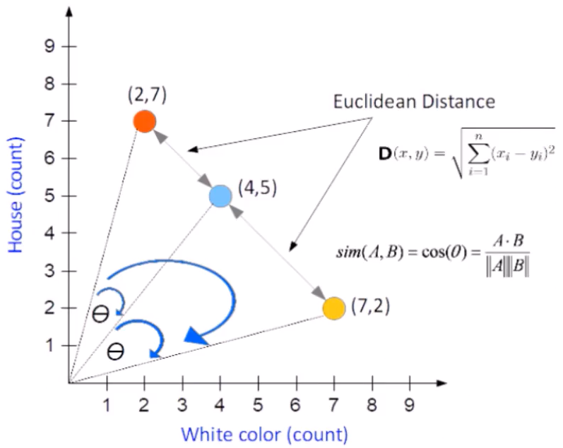
For example, looking at the red point (2,7), 2 is the number of times that the word “white” appears in the text and 7 is the number of times that the word “house” appears in the same text. The blue and yellow points are examples in other texts. Looking at all the points, we have the representation of all text based on their frequency of common words. Now, if we want to evaluate how similar are the text, we can use two different metrics: 1 - Euclidean Distance 2 - Cosine Similarity The cosine similarity is the angle theta between two points. If the theta angle is little, means that the two points are close and as a consequence the two texts are closely related. On the contrary, if the angle is very large, the two texts are not similar. In the formula above, A and B are the vectors (where they start at 0 and arrive to the colored point). The cosine similarity equation will result in a value between 0 and 1. The smaller cosine angle results in a bigger cosine value, indicating higher similarity. In this case Euclidean distance will be zero.
Stemming vs. Lemmatization Stemming is the process of transforming words in their root word, for example: “carefully”, “cared”, “cares” can be considered as ”care” instead of separate words. Lemmatization: we need to have the inflected form of the word. For example the lemmatization of the word “ate” is “eat”. Stemming and Lemmatization both generate the root form of inflected words. The difference is that stem might not be an actual word whereas, lemma is an actual language word. Stemming follows an algorithm with steps to perform on the words which makes it faster. Whereas, in lemmatization, you used WordNet corpus and a corpus for stop words as well to produce lemma which makes it slower than stemming. You also had to define a part-of-speech to obtain the correct lemma.
Minimum edit distance & Backrace method Minimum edit distance allows us to assess how similar two strings are. It is the minimum number of editing operations such as insertion, deletion and substitution that are needed to transform one into the other. As shown above, in order to turn “intention” to “execution” we need to do few edition. If each operation has a cost of 1, the distance between the word “intention” and “execution” is 5. There are lots of distinct paths that wind up at the same state and we don’t have to keep track of all of them. We just need to keep track of the shortest path to each of those revised path. For this reason we can use the Backtrace method.
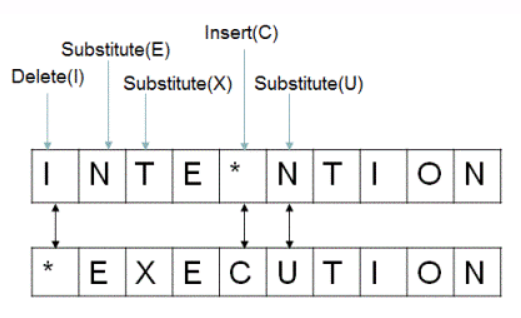
We often need to align each character of the two strings to each other by keeping a backtrace. Every time we enter a cell, we need to remember where we came from and when we reach the end, trace back the path from the upper right corner to read off the alignment. The arrows in the graph below (starting from the upper right corner) allows you to trace back the path. For example, to go from “inte” to “e”, we could remove all 4 characters and insert a letter “e” but that would cost us a distance of 5. Alternatively, we could just remove “int” and get the remainder character “e”, costing us a distance of 3. It is the way to correct grammar errors; maybe not necessary if we are working for example with scientific articles.
Part of speech tag filter - POS In the world of Natural Language Processing (NLP), the most basic models are based on Bag of Words. But such models fail to capture the syntactic relations between words. For example, suppose we build a sentiment analyser based on only Bag of Words. Such a model will not be able to capture the difference between “I like you”, where “like” is a verb with a positive sentiment, and “I am like you”, where “like”" is a preposition with a neutral sentiment. POS tagging is the process of marking up a word in a corpus to a corresponding part of a speech tag, based on its context and definition. For example, in the sentence “Give me your answer”, answer is a Noun, but in the sentence “Answer the question”, answer is a verb. There are different techniques for POS Tagging: 1 - Lexical Based Methods: assigns the POS tag the most frequently occurring in the training corpus. 2 - Rule Based Methods: e.g. the “ed” or “ing” must be assigned to a verb. 3 - Rule Based Method: RNN can be used to solve POS tagging. 4 - Probabilistic Method: assigns the POS tag based on the probability of a particular tag sequence. To have a description of POS look at this link. Every word is represented by a feature tag.
Topic Analysis and LDA Hyperparameters One of he most popular topic algorithm is the LDA. It is of high importance to tune the hyperparameters: 1 - Number of iterations. 2 - Number of Topics: number of topics to be extracted using Kullback Leibler Divergence Score. 3 - Number of Topic Terms: number of terms composed in a single topic. 4 - Alpha hyperparameter: represents document-topic density. 5 - Beta hyperparameter: represent topic-word density. The alpha & beta parameters are especially useful to find the right number of topics. 6 - Batch Wise LDA: another tip to improve the model is to use corpus divided into batches of fixed sizes. We perform LDA on these batches multiple times and we should obtain different results, but strikingly, the best topic terms are always present.
It is often desirable to quantify the difference between probability distributions for a given random variable. The difference between two distribution is called:. statistical distance, but this can be challenging as it can be difficult to interpret the measure. ùin fact, it is more common to calculate a divergence between two probability distributions. Divergence is a scoring of how one distribution differs from another. Two commonly used divergence scores from information theory are Kullback-Leibler Divergence KL and Jensen-Shannon Divergence. The KL divergence between two distributions Q and P is often stated using the following notation: KL(P || Q) where the || operator indicates divergence of P from Q. KL divergence can be calculated as the positive sum of probability of each event in P multiplied by the log of the probability of the event in Q over the probability of the event in P: KL(P || Q) = – sum x in X P(x) * log(Q(x) / P(x)) the value within the sum is the divergence for a given event. The intuition for the KL divergence score is that when the probability for an event from P is large, but the probability for the same event in Q is small, there is a large divergence. When the probability from P is small and the probability from Q is large, there is also a large divergence, but not as large as the first case.
LDA uses some constructs like: 1 - a document can have multiple topics (because of this multiplicity, we need the Dirichlet distribution); and there is a Dirichlet distribution which models this relation. 2 - words can also belong to multiple topics, when you consider them outside of a document; so here we need another Dirichlet to model this. Now, in Bayesian inference you use the Bayes rule to infer the posterior probability. These distributions are hidden from data, this is why is called latent, or hidden.
\[ p(\theta | x)=\frac{p(x | \theta) p(\theta | \alpha)}{p(x | \alpha)} \Longleftrightarrow \text { posterior probability }=\frac{\text { likelihood } \times \text { prior probability }}{\text { marginal likelihood }} \] The alpha parameter in he formula above is our initial belief about this distribution, and is the parameter of the prior distribution. Usually this is chosen in such a way that will have a conjugate prior (so the distribution of the posterior is the same with the distribution of the prior) and often to encode some knowledge if you have one or to have maximum entropy if you know nothing. The parameters of the prior are called hyperparameters. In LDA, both topic distributions, over documents and over words have also correspondent priors, which are denoted usually with alpha and beta, and because are the parameters of the prior distributions are called hyperparameters.
Recommender system in text mining Recommender system is designed to predict the user preference and how to recommend the right items in order to create a user personalization experience. There are two types of recommender system: 1 - Content based filtering: focused on the similarity attributes of the items to give recommendations. 2 - Collaborative filtering: focused on the similarity attribute of the users finding people with similar tastes based on a similarity measure: memory based and model based.
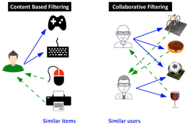
From the figure above, the content based filtering is able to find similar items of the favorite items of the user, such as the mouse and the printer based on the keybord and the joystick. The recommendation is based on the similarity. On the contrary, in the collaborative filtering is focused on the similarity attributes of the users, finding peole with similar traits based on a similarity measure. There are two measures: memory based and model based.
The memory based recommendation is looking items liked by similar people in order to create a ranked list of recommendations. We can sort the ranked list to recommend the top n items to the user. The Person correlation and cosine similarity are used. Here the Pearson correlation formula:
\[ \operatorname{simil}(x, y)=\frac{\sum_{i \in I_{y}}\left(r_{z, i}-\bar{r}_{z}\right)\left(r_{y, i}-\bar{r}_{y}\right)}{\sqrt{\sum_{i \in I_{y}}\left(r_{z, i}-\bar{r}_{z}\right)^{2}} \sqrt{\sum_{i \in I_{y}, i}}\left(r_{y, i}-\bar{r}_{y}\right)^{2}} \]
and the cosine similarity formula:
\[ \operatorname{simil}(z, y)=\cos (\vec{x}, \vec{y})=\frac{\vec{x} \cdot \vec{y}}{|\vec{x}||\times| \vec{y}||}=\frac{\sum_{i \in I_{y}} r_{z, i} r_{y, i}}{\sqrt{\sum_{i \in l_{z}} r_{z, i}^{2}} \sqrt{\sum_{i \in l_{y}} r_{y, i}^{2}}} \] The cosine similiarity formula (see on top of this article) makes sure how to separate two terms where each term is represented by a vector and we are interested in the angle between these two vectors. If the cosine similarity is close to 1, both terms are very similar. In the memory based recommendation the similarity matrix is used.
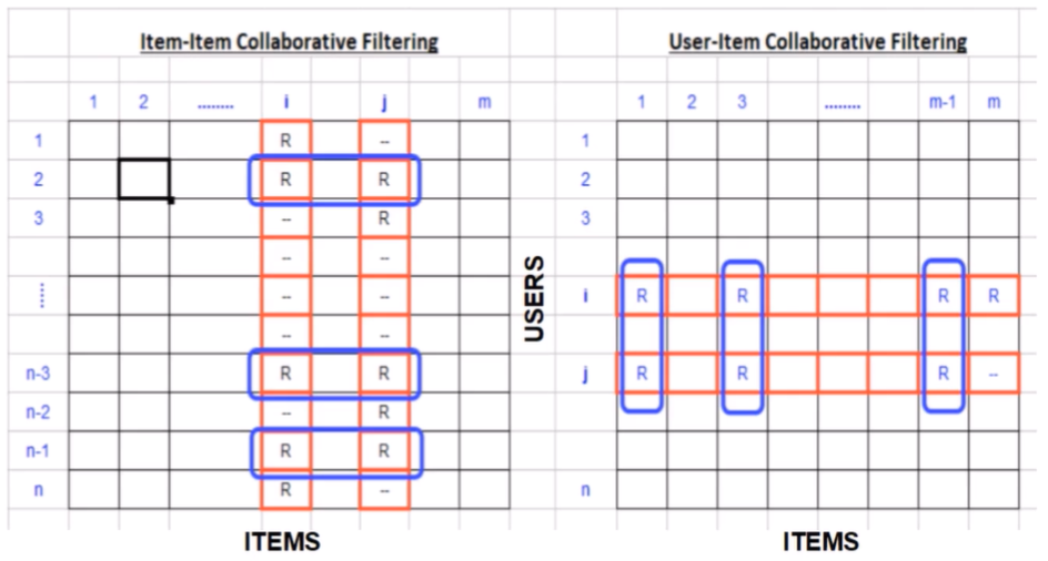
From the figure above we can see on the left the item-item similarity which is calculated by looking into co-ranked items only. Form example, for the items i and j the similarity is computed by calculating similarity between rating the i and j columns (items) but only in the cells where we have a rate (blue rectangles). Another approach is to use the user-item similarity, on the right of the figure above. This approach is looking into correlated items only in rows (users).