The Topic Model is a type of statistical model to find the topics that occur in a collection of documents. It is a frequently used text-mining tool for discovery of hidden semantic structures in a text body. For example, image to have some articles or a series of social media messages and we want to understand what is going on inside of them. A common tool to face this problem is via Unsupervised Machine Learning model. From a high level perspective, having a bunch of documents, and like in K-Mean Clustering we want to find the K number of topics that best describe our corpus of text.
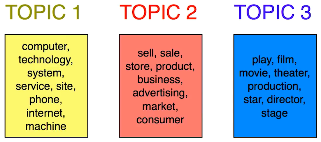
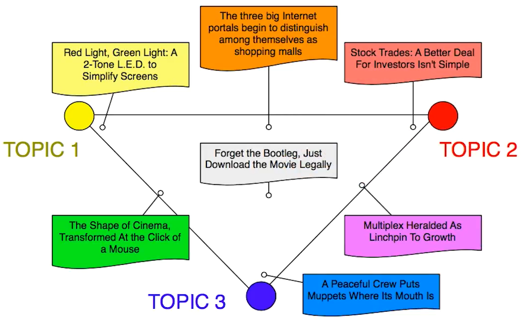
From the figure above, we have three different topics: technology (yellow), business(orange), and arts(blue). In addition to those topics, we also have an association to the documents to topics. In fact, a document can be entirely a technology topic (i.e. red light, green light, 2-tone led, simplify screen), but also a document that is a sort of mixture of two or more topic (see the grey text in the figure below).
Topic Modelcan be seen as a Matrix Factorization Problem, where K is the number of topics, M is the number of documents, and V is the size of the vocabulary.
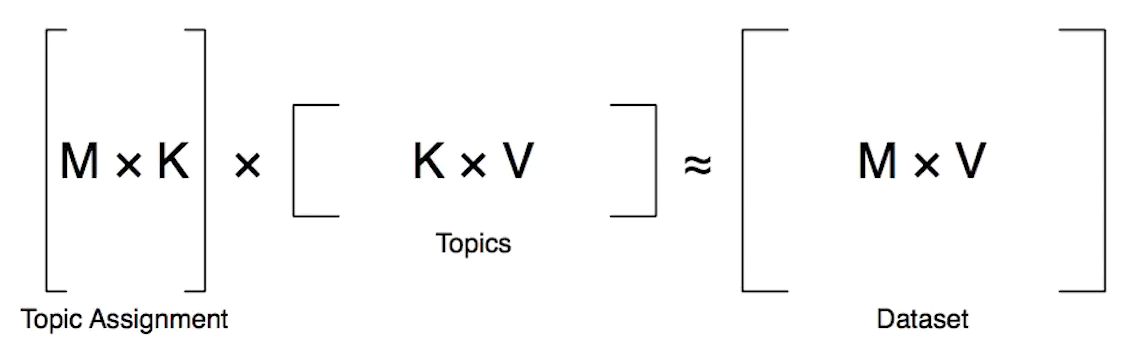
The MxV matrix corresponds to the distribution of the words for each of the topics,and to find this the Latent Semantic Analysis is widely used.
An alternative of the Matrix Factorization Problem is the Generative Model. More particularly, the Latent Dirichlet Allocation is commonly used in topic modelling.
\[ P(\boldsymbol{p} | \alpha \boldsymbol{m})=\frac{\Gamma\left(\sum_{k} \alpha m_{k}\right)}{\prod_{k} \Gamma\left(\alpha m_{k}\right)} \prod_{k} p_{k}^{\alpha m_{k}-1} \]
Here above, we have the Dirichlet Distribution Equation, where alpha is the variance, and m is the mean.
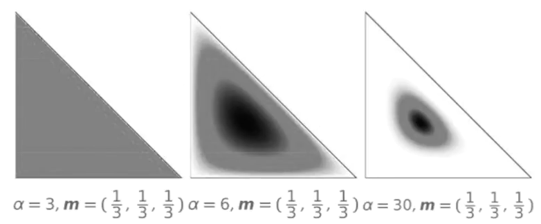
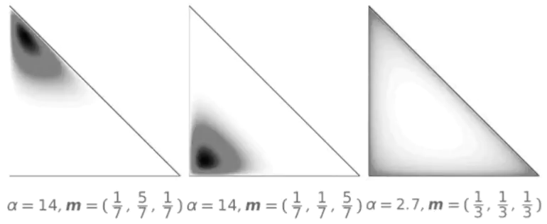
As described in the figure above, when we have a uniform mean (1/3), and an variance (alpha) of three, when we molltiply them togheter, the LDA=1, and so each topic is equally likely. But when the variance is larger and larged the LDA is concentrating the distribution around the mean (the dark circle in the middle of the triangle).
There are other ways to parametrize the LDA distribution. For example, we can have mean in a differnt location (see the left and center figure below). We can also have the variance parameter alpha smaller than 1. In this case we push the probability mass to the edges of the simplex (see the right figure below). In this case, with alpha<1 we have a preference for the multinomial distribution which is far avay for the center. To be far away from the center means we have not a precise topic to assign to our word. It is similar to how people write document where many things are inside a concept. In other words, the Dirichlet Distribution give us a distribution over all the places where the Multinomila Distribution can land.
The Dirichlet Distribution can be used to isolate which document is about a specific topic. For each topic K, we have a multinomial distribution Betak, called Topic Distribution from a Dirichlet Distribution with parameter lambda. The next step is to draw a multinomial distribution over topics represented by Өd. Once we have it, we can draw for each word the so called Topic Assignment represented in the figure below by Zn. Till now, we don’t know what the word is. We have to look at the Topic Distribution Betak in order to generate the word that comes from the multinomial distribution.
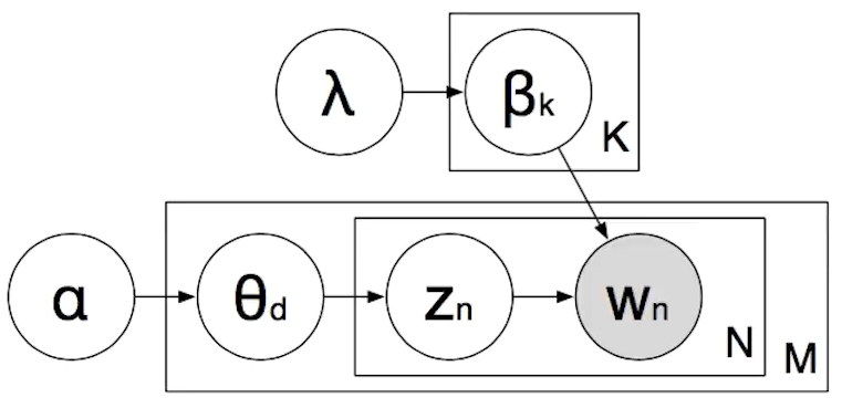
The graph above is a representation of the probabilistic model, also called Plate Notation. As we can see we have in the Plate Notation K topics in M documents, and N words in each document. Crucially, the only thing that we observe are the words, and our task is to figure out what topic to assign Zn.
Ideally, once we have the collection of words per topic, is the topic is interpretable, people will consistently choose true Intruder, or define the words that didn’t belong. To learn more about LDA please check out this link.