Ensemble often have lower error than any individual method by themselves. It has also less overfitting leading us to a better performance in the test set. Each kind of learners that we might use has a sort of bias. Combining all of them, can reduce this bias.
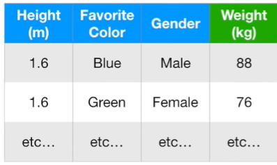
Gradient Boost vs. AdaBoost We start considering to variable reported int he figure below, and we want to predict weight from these variables using decision tree.
Gradient Boost is similar with AdaBoost that starts by building a very short tree called stump from the training data. The amount of say that the stump has on the final output is based on how well the stump compensated for those previous errors. Then the AdaBoost builds the next stump based on the errors that the preavious stump made. In contrast, Gradient Boost starts by making a single leaf instead of a stump. The leaf is an initial guess for the Weight of all the samples. The initial tree is the average value of the independent variable, in this case the average of Weight. Unlike the AdaBoost, the initial tree is larger than a stump: in pratice we set the maximum number of leaves to be between 8 and 32. So, like AdaBoost we have fixed sized trees, but unlike AdaBoost each tree can be larger than a stump. Gradient Boost can be used in Regression and Classification.
Gradient Boost Regression Main Idea The first step is to calculate the average of the independent variable (Weight): this is our first tree. Next, we build a tree baesd on the errors from the first tree (average of Weight) which is the difference betweeb the observed Weight (71.2) and the predicted Weights, and we call there differences Residuals. At this point, we can build the tree based on the dependent variables Height, Favorite Color and Gender.
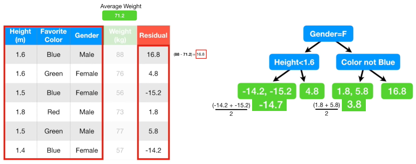
From the figure above, we can see that we used 4 leaves, but is common to use between 8 and 32 leaves. Moreover, we replaced the double residuals by their average, for example: (-14.2-15.2)/2=-14.7 and (1.8+5.8)/2 as we can see from the figure above. The problem of this approach is that we have low Bias but a very high Variance. To deal with this problem Gradient Boost uses a Learning Rate to sclae the contributiion from the new tree. We use a Learning Rate of 0.1 and we do the calculation depicted in the figure below.
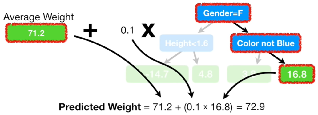
Now, we have a new prediction point of 72.8 for the observed Weith of 88: it is a bit far from the 88 but better than the 71.2 of the first tree made with the average weight. According with Jerome Friedman that invented Gradient Boost: taking lots of small steps in the right direction result in better prediction with the Test Set and this means to have lower Variance.
At this point we can calculate again the Residuals but now using the predicted Weights obtained using the Learning Rate. As we cann see from the figure below, the new residuals are smaller than before.
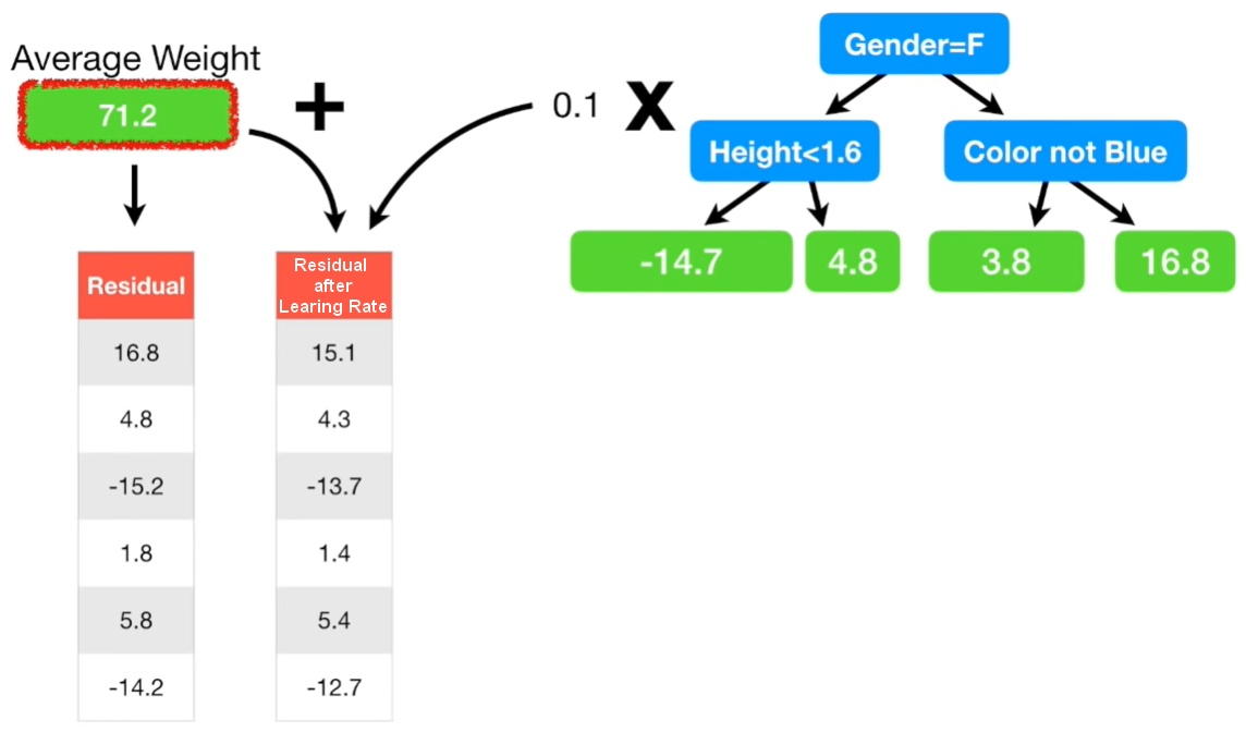
Now, we can calculate the new tree using the new residuals and again with a Learning Rate of 0.1 as we made before. We can sum all the Weights obtained by these trees, and this is a new small step closer to the Observed Weight of 88 kg. As we can see from the figure below, the branches are the same (Gender=F, Height>1.6, Color not Blue), but the leaves are different each time.
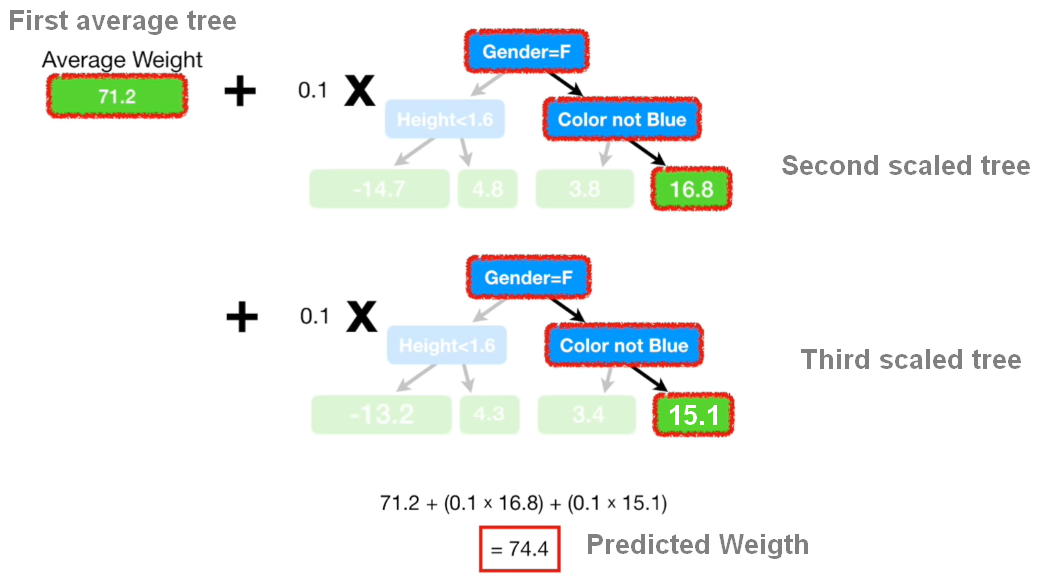
From the figure above, we can see that the step now is to combine the initial avegare tree witht the second and third tree where we scaled the tree by a Learning rate of 0.1. Adding everything together we can predict a new value of Weight of 74.4 which is another step more closer to the Observed Weight of 88 kg.
Crucially, each time we add a tree to the Prediction, the Residuals get smaller, and so we can take another small step (building new tree) towards making a better prediction. So, we keep making trees until we doesn’t significantly reduce the size of the Residuals.
This article is a summary of the StatQuest video made by Josh Starmer. Click here to see the video explained by Josh Starmer.