Empirical Cumulative Distribution Function When summarizing a list of numeric values such as heights, it’s not useful to construct a distribution that assigns a proportion to each possible outcome. It is much more practical to define a function that operates on intervals rather than single values. The standard way of doing this is using the cumulative distribution function (CDF). As an example, we define the empirical cumulative distribution function (eCDF) for heights for male adult students.
library(tidyverse)
library(dslabs)
data("heights")
x <- heights %>% filter(sex=="Male") %>% .$height # take only males

F <- function(a) mean(x<=a) # define the eCDF: that is the probortion of cases equal to a
1 - F(70) # what is the prob. that a male student is higher than 70 inches
[1] 0.3768473Theoretical Distribution The cumulative distribution for the normal distribution is defined by a mathematical formula, which in R can be obtained with the function pnorm. The normal distribution is derived mathematically. Apart from computing the average in the standard deviation, we don’t use data to define it.
1 - pnorm(70, mean(x), sd(x))[1] 0.4247467It does not make sense to ask what is the probability that a normally distributed value is 70. Instead, we define probabilities for intervals. So we could ask instead, what is a probability that someone is between 69.99 and 70.01.
Probability Density The probability density at x is defined as the function, we’re going to call it little f of x, such that the probability distribution big F of a, which is the probability of x being less than or equal to a, is the integral of all values up to a of little f of x dx.
For example, to use the normal approximation to estimate the probability of someone being taller than 76 inches, we can use the probability density.
avg <- mean(x)
s <- sd(x)
1 - pnorm(76, avg, s)
[1] 0.03206008Monte Carlo Simulation We can run Monte Carlo simulations using normally distributed variables. R provides a function to generate normally distributed outcomes. Specifically, the rnorm function takes three arguments size, average, which defaults to 0, standard deviation, which defaults to 1. using the same data used above we can generate the relative normal distribution with the finction rnorm.
x <- heights %>% filter(sex=="Male") %>% .$height
n <- length(x)
avg <- mean(x)
s <- sd(x)

simulated_heights <- rnorm(n, avg, s)

data.frame(simulated_heights=simulated_heights) %>% ggplot(aes(simulated_heights)) +
  geom_histogram(color="black", binwidth = 2)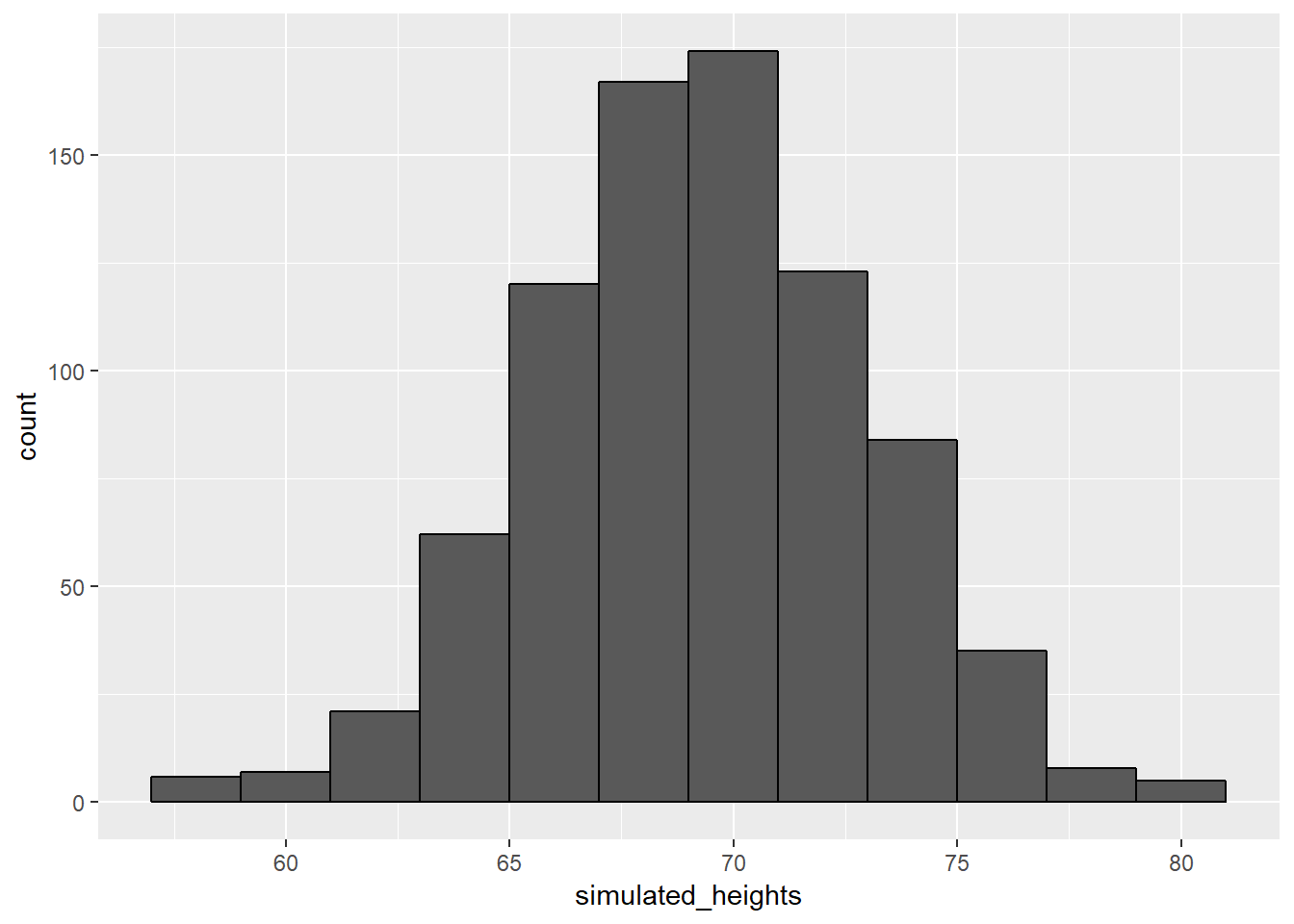
Not surprisingly, the distribution of these outcomes looks normal because they were generated to look normal. This is one of the most useful functions in R, as it will permit us to generate data that mimics naturally occurring events. It’ll let us answer questions related to what could happen by chance by running Monte Carlo simulations. For example, if we pick 800 males at random, what is the distribution of the tallest person? Specifically, we could ask, how rare is that the tallest person is a seven footer?
b <- 10000
tallest <- replicate(b, {
  simulated_data <- rnorm(800, avg, s)
  max(simulated_data)
})

mean(tallest >= 7*12)
[1] 0.0217The normal distribution is not the only useful theoretical distribution. Other continuous distributions that we may encounter are student-t, the chi-squared, the exponential, the gamma, and the beta distribution. R provides functions to compute the density, the quantiles, the cumulative distribution function, and to generate Monte Carlos simulations for all these distributions.
Namely, using the letters d for density, q for quantile, p for probability density function, and r for random. By putting these letters in front of a shorthand for the distribution, gives us the names of these useful functions.
Statistical Inference In data science, we often deal with data that is affected by chance in some way. The data comes from a random sample, the data is affected by measurement error, or the data measures some outcome that is random in nature. Being able to quantify the uncertainty introduced by randomness is one of the most important jobs of a data scientist. For example, in epidemiological studies, we often assume that the subjects in our study are a random sample from the population of interest. Sampling models are therefore ubiquitous in data science. Data scientists talk about what could have been, but after we see what actually happened.