The Quantile regression gives a more comprehensive picture of the effect of the independent variables on the dependent variable. Instead of estimating the model with average effects using the OLS linear model, the quantile regression produces different effects along the distribution (quantiles) of the dependent variable. The dependent variable is continuous with no zeros or too many repeated values. Examples include estimating the effects of household income on food expenditures for low- and high-expenditure households, what are the factors influencing total medical expenditures for people with low, medium and high expenditures. The following oexample is based on Medical Expenditure Panel Survey MEPS. The dependent variable is the total medical expenditures, and the independent variables are: supplemental insurance, total number of chronic conditions, age, female, and white. We estimate an OLS regression, and quantile regression at 25th, 50th, and 75th quantile. The standard Ordinary Least Squares OLS models the relationship between one or more independent variables and the conditional mean of a dependent variable. The Quantile Regression models the relationship betwwn the conditional quantiles rather than just the conditional mean of the dependent variable. A quantile regression gives a more comprehensive picture of the effect of the independent variables on the dependent variable because we can show different effects (quantiles). One pratical consideration is that the distribution of the dependent variable has to be continuous and it shouldn’t has zero or too many repeated values. One important aspect to take in considertion in Quantile Regression is that coefficients can be significanlty different than the OLS coefficients, showing different effects along the distribution of the dependent variable. The advantages of the Quantile regression are: Flexibility for modeling data with heterogeneous conditional distributions. Median regression is more robust to outliers than the OLS regression. Quantile regression can show different effects of the independent variables on the dependent variable depending across the spectrum of the dependent variable.
library(quantreg)
mydata <- read.csv("C:/07 - R Website/dataset/ML/quantile_health.csv")
attach(mydata)
summary(mydata)
dupersid totexp ltotexp suppins
Min. :20004018 Min. : 3 Min. : 1.099 Min. :0.0000
1st Qu.:24476022 1st Qu.: 1433 1st Qu.: 7.268 1st Qu.:0.0000
Median :90123058 Median : 3334 Median : 8.112 Median :1.0000
Mean :62616065 Mean : 7290 Mean : 8.060 Mean :0.5915
3rd Qu.:94161512 3rd Qu.: 7492 3rd Qu.: 8.922 3rd Qu.:1.0000
Max. :98347025 Max. :125610 Max. :11.741 Max. :1.0000
totchr age female white
Min. :0.000 Min. :65.00 Min. :0.0000 Min. :0.0000
1st Qu.:1.000 1st Qu.:69.00 1st Qu.:0.0000 1st Qu.:1.0000
Median :2.000 Median :74.00 Median :1.0000 Median :1.0000
Mean :1.809 Mean :74.25 Mean :0.5841 Mean :0.9736
3rd Qu.:3.000 3rd Qu.:79.00 3rd Qu.:1.0000 3rd Qu.:1.0000
Max. :7.000 Max. :90.00 Max. :1.0000 Max. :1.0000 # Define variables
Y <- cbind(totexp)
X <- cbind(suppins, totchr, age, female, white)The variable totexp is the total expenditure and is dependent variable. The independent variables are suppins supplemental insurance, totchr total number of chronic conditions, age, female, and white. The first step is to perform an OLS regression.
# OLS regression
olsreg <- lm(Y ~ X, data=mydata)
summary(olsreg)
Call:
lm(formula = Y ~ X, data = mydata)

Residuals:
   Min     1Q Median     3Q    Max
-16146  -5372  -2804    457 115461

Coefficients:
             Estimate Std. Error t value Pr(>|t|)
(Intercept)   461.492   2777.453   0.166  0.86805
Xsuppins      585.984    436.309   1.343  0.17936
Xtotchr      2528.079    164.834  15.337  < 2e-16 ***
Xage            6.711     33.768   0.199  0.84248
Xfemale     -1239.866    433.110  -2.863  0.00423 **
Xwhite       2193.155   1327.794   1.652  0.09870 .
---
Signif. codes:  0 '***' 0.001 '**' 0.01 '*' 0.05 '.' 0.1 ' ' 1

Residual standard error: 11520 on 2949 degrees of freedom
Multiple R-squared:  0.07828,   Adjusted R-squared:  0.07672
F-statistic: 50.09 on 5 and 2949 DF,  p-value: < 2.2e-16
The Xtotchr, the total of chronic condition, says that each of chronich condition brings 2528.079 more dollars in totexp total medical expenditure. Now, we perform a quantile regression.
# Simultaneous quantile regression
quantreg2575 <- rq(Y ~ X, data=mydata, tau=c(0.25, 0.75))
summary(quantreg2575)
Call: rq(formula = Y ~ X, tau = c(0.25, 0.75), data = mydata)

tau: [1] 0.25

Coefficients:
            Value       Std. Error  t value     Pr(>|t|)
(Intercept) -1412.88889   433.20179    -3.26150     0.00112
Xsuppins      453.44444    75.05348     6.04162     0.00000
Xtotchr       782.47222    37.55769    20.83388     0.00000
Xage           16.08333     6.19162     2.59760     0.00943
Xfemale        16.05556    72.20278     0.22237     0.82404
Xwhite        338.08333    71.51522     4.72743     0.00000

Call: rq(formula = Y ~ X, tau = c(0.25, 0.75), data = mydata)

tau: [1] 0.75

Coefficients:
            Value       Std. Error  t value     Pr(>|t|)
(Intercept) -4512.04545  2350.56284    -1.91956     0.05501
Xsuppins      708.40909   375.76929     1.88522     0.05950
Xtotchr      2855.31818   196.12587    14.55860     0.00000
Xage           87.36364    30.98410     2.81963     0.00484
Xfemale      -554.59091   378.71501    -1.46440     0.14319
Xwhite        801.68182   370.96108     2.16109     0.03077
The Xtotchr, the total of chronic condition, for the 0.25 quantile is 782.47, and the interpretatation is: adding 25th quantile each of chronich condition brings only 782.42 more dollars in totexp total medical expenditure. This is a much ower value that we had before with OLS. This means, for low number of chronic conditions the medical expenditure is lower. On the oder hand, looking at the 0.75 quantile for the total of chronic condition we have 2855.31 more dollar per each more chronic condition. This value is more similar with the OLS coefficient, and in fact this time we have not a significant difference from the OLS coefficient.
We can also perform an ANOVA to compare the coefficient at 25th quantile vs. 75th quantile.
# Quantile regression at 25 the quanile
quantreg25 <- rq(Y ~ X, data=mydata, tau=0.25)

# Quantile regression at 75 the quanile
quantreg75 <- rq(Y ~ X, data=mydata, tau=0.75)

# ANOVA test for coefficient differences
anova(quantreg25, quantreg75)
Quantile Regression Analysis of Deviance Table
Model: Y ~ X
Joint Test of Equality of Slopes: tau in { 0.25 0.75 }
Df Resid Df F value Pr(>F)
1 5 5905 37.831 < 2.2e-16 ***
---
Signif. codes: 0 '***' 0.001 '**' 0.01 '*' 0.05 '.' 0.1 ' ' 1As we can see from the result above, there is a significant difference in the coefficients, and this justify to use the quantile regression. Now, we can plot the data and the coefficinets we found from the quantile regression.
# Plotting data
quantreg.all <- rq(Y ~ X, tau = seq(0.05, 0.95, by = 0.05), data=mydata)
quantreg.plot <- summary(quantreg.all)
plot(quantreg.plot)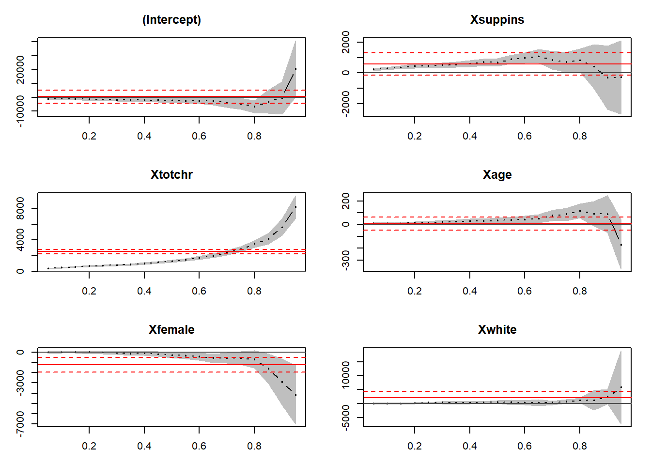
We focus our attention on the Xtotchr (total of chronic condition) graph. The red orizontal line is the OLS coefficient, and we can see that the value is exactly the same of what we found before (2528.079). Notice that the OLS line is flat along the quantile in the x-axis, because it cannot vary across the quantiles. Looking at the quantile trend (black curve with grey confidence intervals), we can see that for low quantiles there is a significant difference below OLS. On the contrary, there is a significant difference above OLS for high quantile. Again, we can see from the graph of Xtotchr that there is not a significant difference for the 75th quantile.
Looking at the Xage graph, there is not a significat difference from OLS across the quantiles, except at the last quantile.