Principal Component Analysis PCA is a deterministic method (given an input will always produce the same output). It is always good to perform a PCA: Principal Components Analysis (PCA) is a data reduction technique that transforms a larger number of correlated variables into a much smaller set of uncorrelated variables called PRINCIPAL COMPONENTS. For example, we might use PCA to transform many correlated (and possibly redundant) variables into a less number of uncorrelated variables that retain as much information from the original set of variables.
data(iris)
summary(iris)
Sepal.Length Sepal.Width Petal.Length Petal.Width
Min. :4.300 Min. :2.000 Min. :1.000 Min. :0.100
1st Qu.:5.100 1st Qu.:2.800 1st Qu.:1.600 1st Qu.:0.300
Median :5.800 Median :3.000 Median :4.350 Median :1.300
Mean :5.843 Mean :3.057 Mean :3.758 Mean :1.199
3rd Qu.:6.400 3rd Qu.:3.300 3rd Qu.:5.100 3rd Qu.:1.800
Max. :7.900 Max. :4.400 Max. :6.900 Max. :2.500
Species
setosa :50
versicolor:50
virginica :50
We are using the iris dataset with 4 numerical variables and 1 factor which has 3 levels as described above. We can also see that the numerical variables have different ranges, it is a good pratice to normalize the data.
# Partition Data
set.seed(111)
ind <- sample(2, nrow(iris),
              replace = TRUE,
              prob = c(0.8, 0.2))

training <- iris[ind==1,]
testing <- iris[ind==2,]

# Scatter Plot & Correlations
library(psych)
pairs.panels(training[,-5], # not use the factor variable
             gap = 0,       # is the gap between the scatterplot
             bg = c("red", "yellow", "blue")[training$Species],
             pch=21)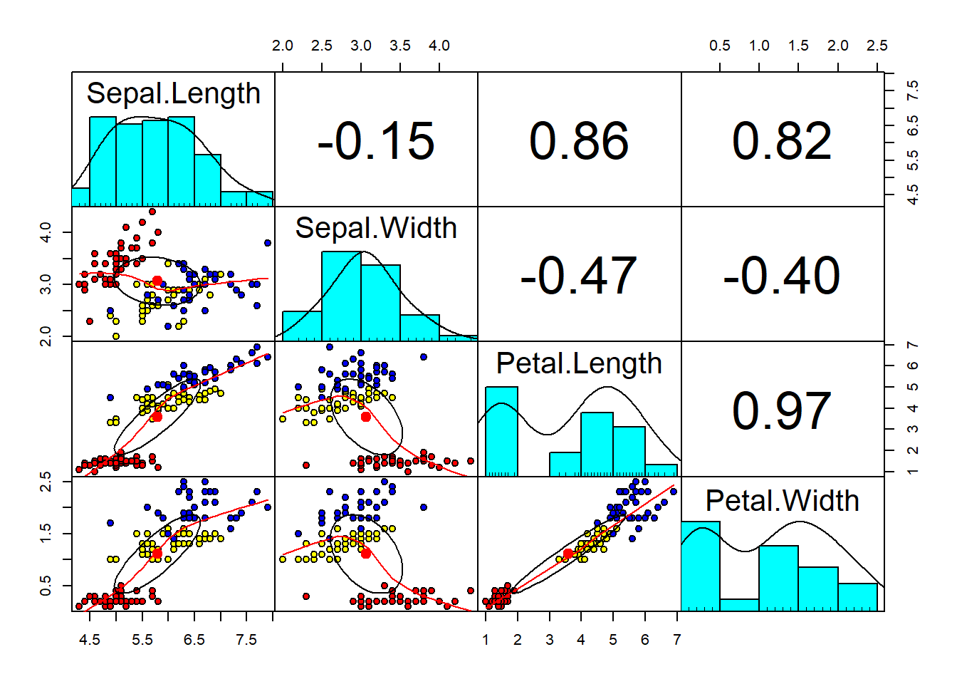
As we can see above, we have the correlation among the variables in the training data. We also colored the observations based on species (setosa, versicolor, virginica). On the upper corner we can also see the correlation coefficient, and in the main diagonal the distribution of the variables. It is evident here that Petal.Length and Petal.Width are positive correlated with an R-squared of 0.97, very closed to 1. On the other hand, we see a correlation almost close to 0 between Sepal.Length and Sepal.Width. Overall, in three cases we have very high correlations. High correlations among independent variables lead to Multicollinearity problem. It is the phenomenon in which one predictor can be linearly predict from others with a substantial degree of accuracy. In this situation, the coefficients estimated may change erratically in response to small changes of the model. To prevent it, one of the approches is the PCA.
# Principal Component Analysis
pc <- prcomp(training[,-5],
             center = TRUE, # convert the data in order to have an average of zero
             scale. = TRUE) # before pca normalize the variales

# attributes(pc) # see attributes
# pc$center
# pc$scale
print(pc) # show sd and loadings
Standard deviations (1, .., p=4):
[1] 1.7173318 0.9403519 0.3843232 0.1371332
Rotation (n x k) = (4 x 4):
PC1 PC2 PC3 PC4
Sepal.Length 0.5147163 -0.39817685 0.7242679 0.2279438
Sepal.Width -0.2926048 -0.91328503 -0.2557463 -0.1220110
Petal.Length 0.5772530 -0.02932037 -0.1755427 -0.7969342
Petal.Width 0.5623421 -0.08065952 -0.6158040 0.5459403summary(pc)Importance of components:
PC1 PC2 PC3 PC4
Standard deviation 1.7173 0.9404 0.38432 0.1371
Proportion of Variance 0.7373 0.2211 0.03693 0.0047
Cumulative Proportion 0.7373 0.9584 0.99530 1.0000Using the function print(pc) we can see the standard deviation and also the Loading Score (in the resul above are called Rotation): from the distance on x axis and the distance from y axis is possible to use the Pythagorean Theorem to find the hypotenuse of each observation and we scale it to a unit of one: this is called Singular Vector or Eigenvector for Principal Component One. This calculation that we make for all the observations is called Loading Scores. The square root of the eigenvector for PC1 is called the Singular Value for PC1. Moreover, from the summary(pc) we have the standard deviation, and the Proportional of Variance that says PC1 explain the 73.73% of the variability. The second principal component PC2 captures the 22.11% of the variability. From the Cumulative Proportion, at the PC2 we reach 96.84%, and so more than 95% of the variability has been explained. This allow us to exclude PC3 and PC4. Now, we can plot the four principal component and look at their correlation.
# Orthogonality of PCs
pairs.panels(pc$x, # x is the plae where pc is stored
             gap=0,
             bg = c("red", "yellow", "blue")[training$Species],
             pch=21)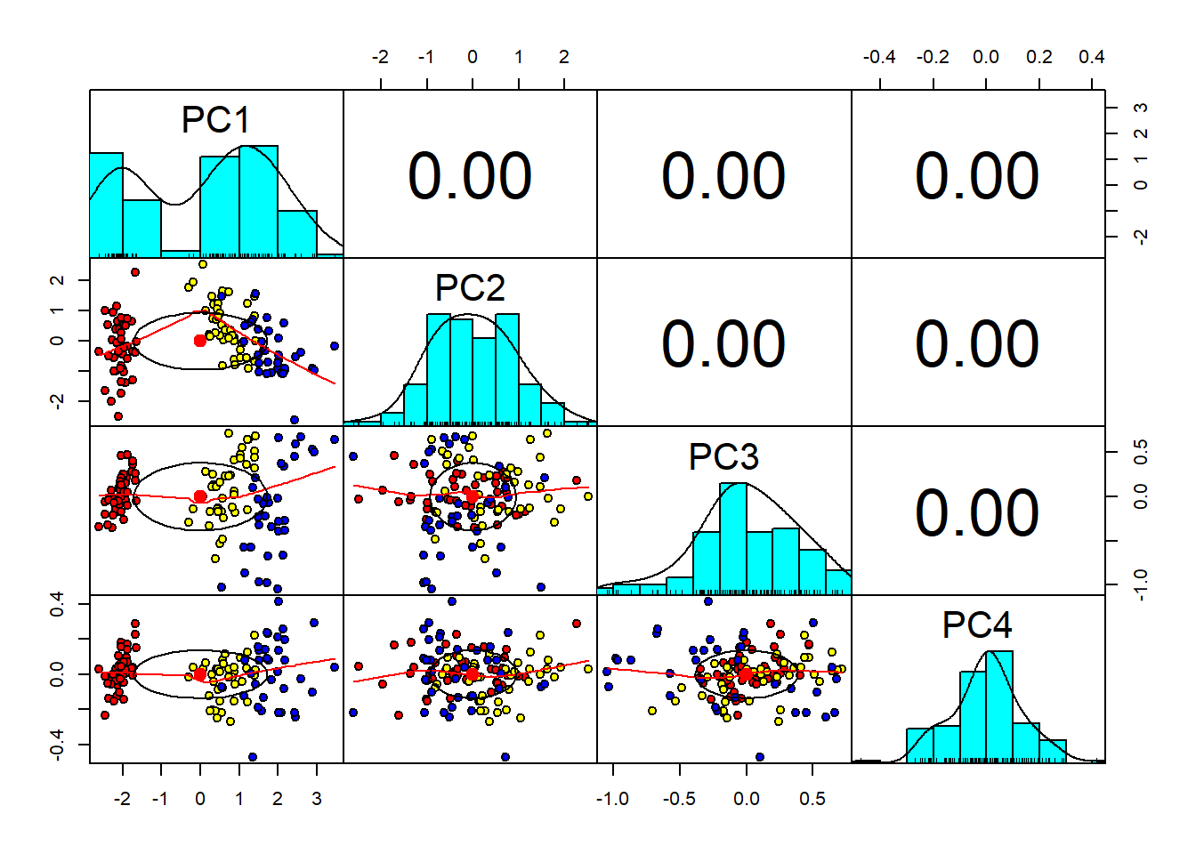
As we can see from the graph above, the four Principal Component, all the correlation coefficients are zero, and so each principal component are ortogonal to each other. Now, we can use the Bi-Plot which is a generalization of the simple two-variable scatterplot, and shows how strongly each characteristic influences a principal component.
# Bi-Plot
library(devtools)
# install_github("ggbiplot", "vqv")
library(ggbiplot)
g <- ggbiplot(pc,
              obs.scale = 1,
              var.scale = 1,
              groups = training$Species,
              ellipse = TRUE,
              circle = TRUE,
              ellipse.prob = 0.68)
g <- g + scale_color_discrete(name = '')
g <- g + theme(legend.direction = 'horizontal',
               legend.position = 'top')
print(g)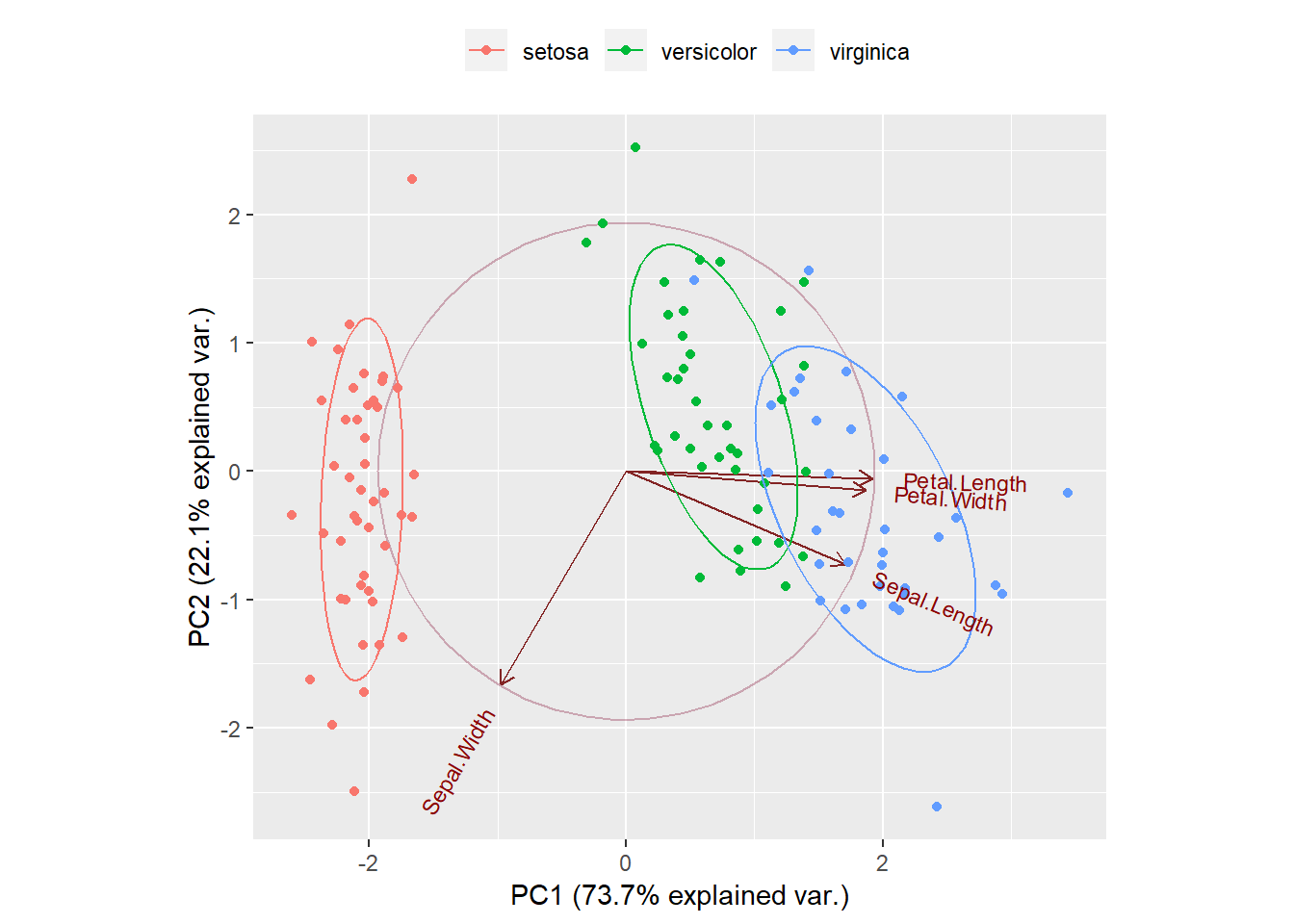
From the Bi-Plot above we have PCA on the x-axis and PC2 on the y-axis. The ellipses explain us the each species (setosa, versicolor, virginica) capture 68% of the data. Within the main circle there are arrows representing the features of out dataset. We can see that Petal.Length and Petal.With have high correlation and they are also correlated with Sepal.Length. On the contrary, Sepal.Width is far away from the other features. If we look at the x-axis, we have Petal.Length, Petal.With, and Sepal.Length on the right side, at a positive value of 2, and this means that these variables are positive correlated.
# Prediction with Principal Components
trg <- predict(pc, training)
trg <- data.frame(trg, training[5])
tst <- predict(pc, testing)
tst <- data.frame(tst, testing[5])
Now we have the data ready for the model, and in this case we use a Multinomial Logistic Regression using the first two Principal Components. We use only PC1 and PC2 because we have more than 95% of the variability capture. Multinomial logistic regression (often just called ‘multinomial regression’) is used to predict a nominal dependent variable given one or more independent variables. It is sometimes considered an extension of binomial logistic regression to allow for a dependent variable with more than two categories.
# Multinomial Logistic regression with First Two PCs
library(nnet)
trg$Species <- relevel(trg$Species, ref = "setosa")
mymodel <- multinom(Species~PC1+PC2, data = trg)
# weights: 12 (6 variable)
initial value 131.833475
iter 10 value 20.607042
iter 20 value 18.331120
iter 30 value 18.204474
iter 40 value 18.199783
iter 50 value 18.199009
iter 60 value 18.198506
final value 18.198269
convergedsummary(mymodel)Call:
multinom(formula = Species ~ PC1 + PC2, data = trg)
Coefficients:
(Intercept) PC1 PC2
versicolor 7.2345029 14.05161 3.167254
virginica -0.5757544 20.12094 3.625377
Std. Errors:
(Intercept) PC1 PC2
versicolor 187.5986 106.3766 127.8815
virginica 187.6093 106.3872 127.8829
Residual Deviance: 36.39654
AIC: 48.39654 If we look at the summary above, we have the intercept and coefficients,and now we can look at the performance via confusion matrix.
# Confusion Matrix & Misclassification Error - training
p <- predict(mymodel, trg)
tab <- table(p, trg$Species)
tab
p            setosa versicolor virginica
  setosa         45          0         0
  versicolor      0         35         3
  virginica       0          5        32
1 - sum(diag(tab))/sum(tab)[1] 0.06666667# Confusion Matrix & Misclassification Error - testing
p1 <- predict(mymodel, tst)
tab1 <- table(p1, tst$Species)
tab1
p1           setosa versicolor virginica
  setosa          5          0         0
  versicolor      0          9         3
  virginica       0          1        12
1 - sum(diag(tab1))/sum(tab1)[1] 0.1333333From the confusion matrix of the training set we have 3 missclassification for versicolor and 5 missclassification for virginica,and so we have an overall missclassification of 0.066%. For the test set the missclassification is a bit higher.
Summarizing, the advantages of PCA are: 1 - Useful for dimension reduction for high-dimentional data analysis. 2 - Help to reduce the number of predictor items using principal components. 3 - Helps to make predictor items independent and avoid multicollinearity problem. 4 - Allows interpretation of many variables using a 2-dimensional biplot. 5 - Can be used for developing prediction models.
The disadvantages of PCA are: 1 - Only numeric variables can be used. 2 - Prediction models are less interpretable.