Polynomial Linear Regression Polynomial Linear Regression fits a nonlinear relationship between the value of x and the corresponding conditional mean of y, and has been used to describe nonlinear phenomena such as the progression of disease epidemics. Although polynomial regression fits a nonlinear model to the data, as a statistical estimation problem it is linear, in the sense that the regression function is linear in the unknown parameters that are estimated from the data. It is a linear conbination of coefficients that are unknowns. For this reason, polynomial regression is considered to be a special case of multiple linear regression. How to find the best fitting live from the graph above is the linear model method.
library(ggplot2)
dat <- read.csv("C:/07 - R Website/dataset/ML/Dat.csv", sep = ";")

# Linear regression
lm(y ~ x, data=dat)
Call:
lm(formula = y ~ x, data = dat)

Coefficients:
(Intercept)            x
     -65.27        34.04
Having the coefficinet of the linear model, calculated above, we can plot the trend line.
f <- function(x){
     return(34.04*x-65.27)
}

ggplot() +
  geom_point(data=dat, aes(x=x, y=y)) +
  stat_function(data=data.frame(x=c(-5,15)), aes(x=x), fun=f) # define left and right extremes of the dataframe and plot the function f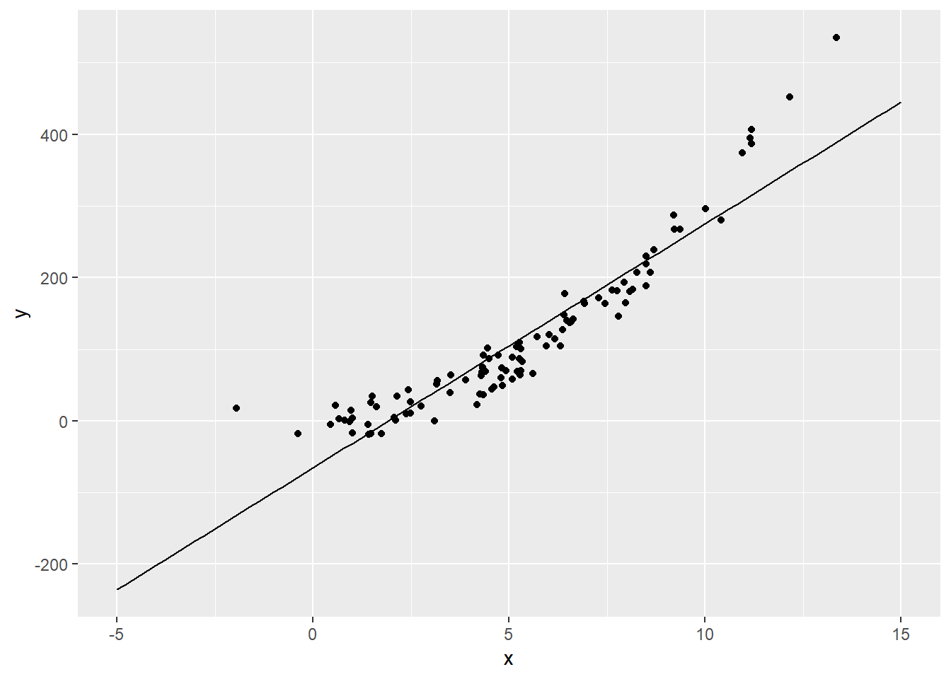
Now that we have the linear trend, we can go along the least squares line, and for each we get the point that correspond to it on the trend line.
x <- dat$x
y <- f(x) # f is the function defined above based on the fitting line
means <- data.frame(x,y) # create a data frame with values of x and the fitted values of y

dat$group <- 1:100 # create a vectro from 1 to 100
means$group <- 1:100 # create a vectro from 1 to 100
groups <- rbind(dat, means)


# Add the fitted point to the graph
ggplot() +
  geom_point(data=dat, aes(x=x, y=y)) +
  stat_function(data=data.frame(x=c(-5,15)), aes(x=x), fun=f) + # define left and right extremes of the dataframe and plot the function f
  geom_point(data=means, aes(x=x, y=y), color='red', size=2) + # add the fitted data points
  geom_line(data=groups, aes(x=x, y=y, group=group))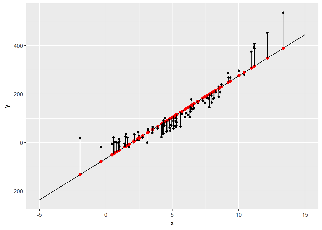
# Calculate the Sum of the Square Residual
sum((dat$y-means$y)^2)
[1] 158423.5The distances that we plotted above are the residuals, and if we want to understand how well the trend line fits the data, we have to square ech of the black lines (residuals) shown in the graph above, then sum up all of them and this process is called Resuduals Sum of Square. From this calculation we found 158423.5 which is a very high value. We can try to fit another kind of polynomium, but not a line in order to get a better fit. So, now we try to fit a quadratic polynomium and a polynomial of degree three.
# Second degree polynomium
lm(y ~ x + I(x^2), data=dat)
Call:
lm(formula = y ~ x + I(x^2), data = dat)

Coefficients:
(Intercept)            x       I(x^2)
    -0.5685       0.9719       2.9522
# Define a function for the polynomial
f <- function(x){
return(2.9522*x^2+0.9719*x-0.5685)
}
means$y <- f(means$x) # calculate fitted points
groups <- rbind(dat, means)
# Add the fitted point to the graph and the residual lines
ggplot() +
geom_point(data=dat, aes(x=x, y=y)) +
stat_function(data=data.frame(x=c(-5,15)), aes(x=x), fun=f) + # define left and right extremes of the dataframe and plot the function f
geom_point(data=means, aes(x=x, y=y), color='red', size=2) + # add the fitted data points
geom_line(data=groups, aes(x=x, y=y, group=group))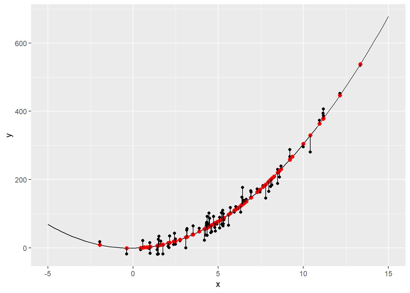
# Calculate the Sum of the Square Residual
sum((dat$y-means$y)^2)
[1] 34582.44as we can see above, now we have a mich smaller Sum of the Square Residuals equal to 34582.44, and this is a much better fit. Now we can try to add one more degree and create a polynomial of degree three.
# Third degree polynomium
lm(y ~ x + I(x^2) + I(x^3), data=dat)
Call:
lm(formula = y ~ x + I(x^2) + I(x^3), data = dat)

Coefficients:
(Intercept)            x       I(x^2)       I(x^3)
   -1.67268      2.49528      2.60142      0.02024
# Define a function for the third degree polynomial
f <- function(x){
return(0.02024*x^3 + 2.60142*x^2 + 2.49528*x -1.67268)
}
means$y <- f(means$x) # calculate fitted points
groups <- rbind(dat, means)
# Calculate the Sum of the Square Residual
sum((dat$y-means$y)^2)[1] 34483.81# Add the fitted point to the graph and the residual lines
ggplot() +
geom_point(data=dat, aes(x=x, y=y)) +
stat_function(data=data.frame(x=c(-100,50)), aes(x=x), fun=f) + # define left and right extremes of the dataframe and plot the function f
geom_point(data=means, aes(x=x, y=y), color='red', size=2) + # add the fitted data points
geom_line(data=groups, aes(x=x, y=y, group=group))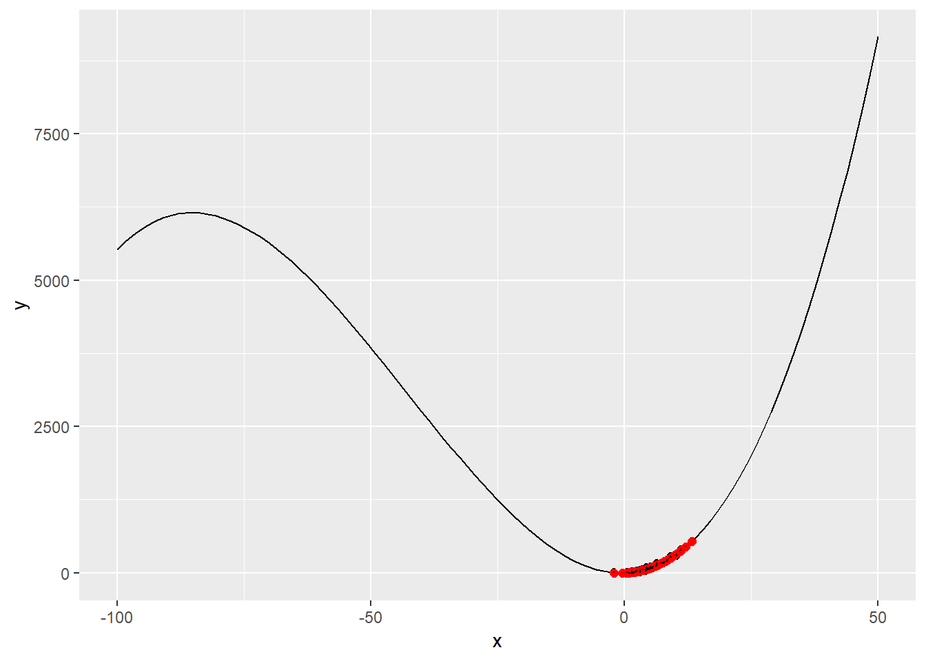
From the code above, we can see that now with a thidr degree polynomial the Sum of the Square Residuals 34483.81, is almost the same then before with the second degree polynomial, just slightly better. From the graph now we can see the cubit shape. What could we do now, is to get even better fit using cubic spline.
Smoothing Spline Instead of fitting a third degree polynomial to all of the data points we are zooming into a small regini of hte points and fitting a cubic polynomial there. Then, we moving on into a next small region and again we ftt a cubic polynomial. At the end we connect these little cubic polynomials so that we end up with a continuous smooth curve through the points. The main difference between polynomial and spline is that polynomial regression gives a single polynomial that models your entire data set. Spline interpolation, however, yield a piecewise continuous function composed of many polynomials to model the data set.
library(splines)

# Define smooth spline
fit <- smooth.spline(dat$x, dat$y, df=50) # put a value for degrees of freedom that control the rough of the curve

# Define a function for the snoooth spline
f <- function(x){
     return(predict(fit,x)$y)
}

# Calculate fitted points
means$y <- predict(fit,means$x)$y

# Calculate the Sum of the Square Residual
sum((dat$y-means$y)^2)
[1] 14244.2# Add the fitted point to the graph
ggplot() +
geom_point(data=dat, aes(x=x, y=y)) +
stat_function(data=data.frame(x=c(-2,14)), aes(x=x), fun=f) + # define left and right extremes of the dataframe and plot the function f
geom_point(data=means, aes(x=x, y=y), color='red', size=2)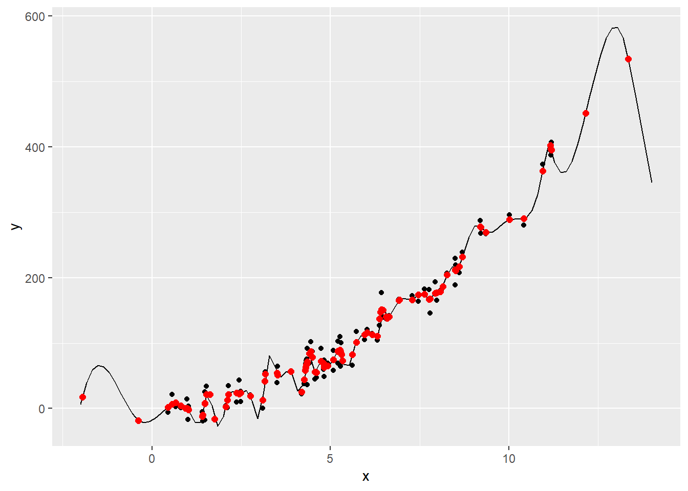 As we can see, now the Sum of the Square Residuals is drammatically decrease to 14244.2, and the more wiggly is the trend curve. Now the trend curve is really trying to follow the data points. This is not a good thing, we have not to care about how well our model or our curve fits the data, because we have to care about of the data that we get in the future. In the quadratic polynomial the model tend to follow the general shape of the dataset. On the oher hand if we look at the smooth spline with 50 degree of freedom, we are going away from falling just the general shape of the data. In other words, we are starting to follow the randomness of the data. This lead us to a very bad prediction because is too tied to the specific data points. The quadratic function is the best solition in accordance with the Principle of Parsimony that says: simpler solutions are more likely to be correct than complex ones. On the contrary the the smooth spline with 50 degree of freedom is an example of Overfitting, and this is definitely a danger to avoided.