Naive Bayes is an effective and commonly-used, machine learning classifier. It is a probabilistic classifier that makes classifications using the Maximum A Posteriori decision rule in a Bayesian setting. It can also be represented using a very simple Bayesian network. Naive Bayes classifiers have been especially popular for text classification, and are a traditional solution for problems such as spam detection.
An intuitive explanation for the Maximum A Posteriori Probability MAP is to think probabilities as degrees of belief. For example, how likely are we vote for a candidate depends on our prior belief. We can modify our stand based on the evidence. Our final decision, based on evidence, is the posterior belief, which is what happens after we sifted through the evidence. MPA is simply the maximum posterior belief: after going through all the debates, what is your most likely decision.
We use Naive Bayes in an example to predict, based on some features (e.g. the rank of the school student come from), if a student is admitted or rejected.
library(naivebayes)
library(dplyr)
library(ggplot2)
library(psych)
data <- read.csv("C:/07 - R Website/dataset/ML/binary.csv")
data$rank <- as.factor(data$rank)
data$admit <- as.factor(data$admit)

# Visualization
pairs.panels(data[-1])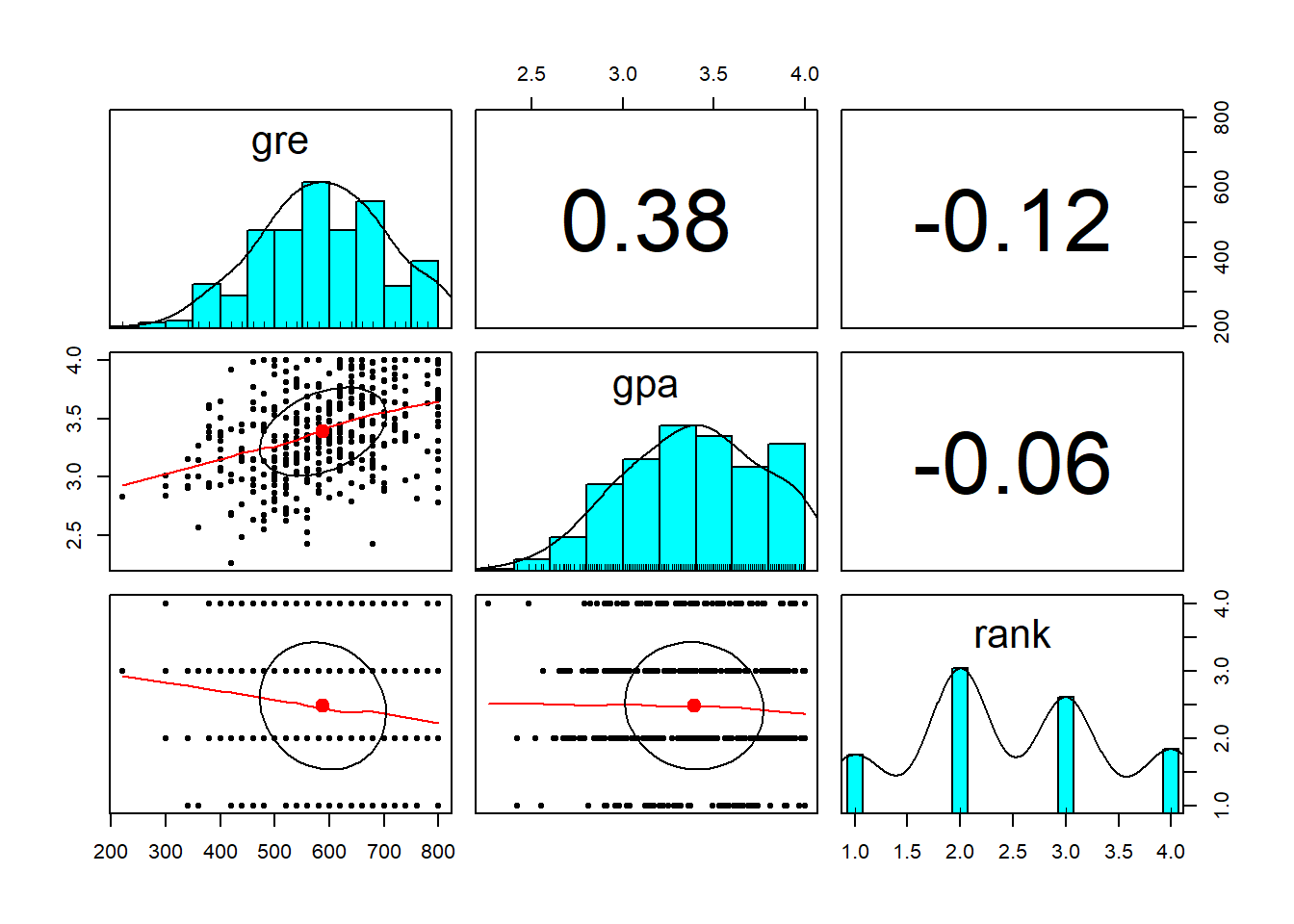
data %>%
  ggplot(aes(x=admit, y=gre, fill=admit)) +
  geom_boxplot()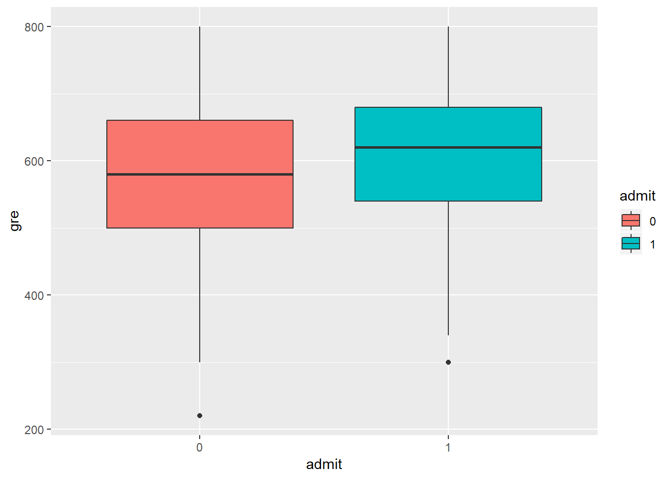
data %>%
ggplot(aes(x=gre, fill=admit)) +
geom_density(alpha=0.8, color='black')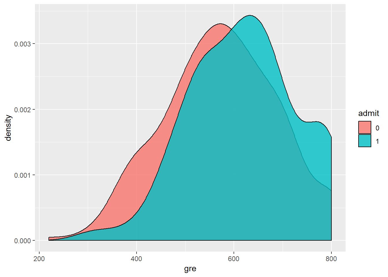 In order to develop a model, we have to make sure that the independent variables are not highly correlated. We can see from the scatterplot above that the only numerical variables are gre and gpa, and they are not strogly correlated (R-squared=0.38). Moreover, looking at the boxplot that compare admit as a function of gre, there is a significant overlap between the two levels of admit. From the dnsity plot of gre as a function on admit, we can see that students not admitted (admit=1) have higher gre comapared to student admitrìted (admit=0). Anyway, there is a significat amount of overlap between the two distributioins. The same is for gpa, here not shown.
# Data Preparation
set.seed(1234)
ind <- sample(2, nrow(data), replace=TRUE, prob = c(0.8, 0.2))
train <-data[ind == 1,]
test <-data[ind == 2,]
Now, the probability of a student admitted given he belongs to rank one: p(admit=1|rank=1) is equal to: **p(admit=1)*p(rank=1|admit=1)/p(rank=1)**
# Naive Bayes Model
model <- naive_bayes(admit ~ ., data = train)
model
================================ Naive Bayes =================================
Call:
naive_bayes.formula(formula = admit ~ ., data = train)
A priori probabilities:
0 1
0.6861538 0.3138462
Tables:
gre 0 1
mean 578.6547 622.9412
sd 116.3250 110.9240
gpa 0 1
mean 3.3552466 3.5336275
sd 0.3714542 0.3457057
rank 0 1
1 0.10313901 0.24509804
2 0.36771300 0.42156863
3 0.33183857 0.24509804
4 0.19730942 0.08823529plot(model)
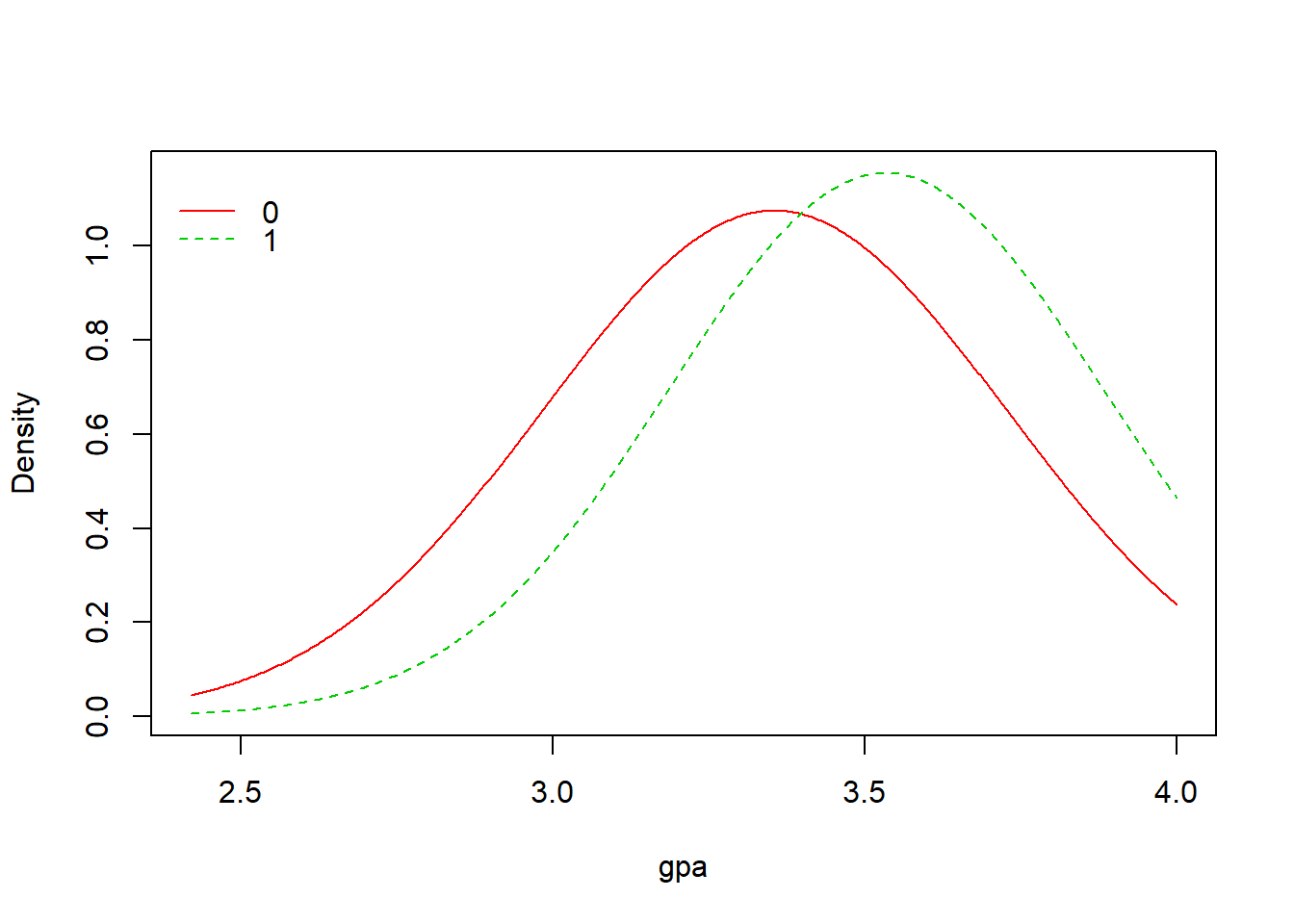
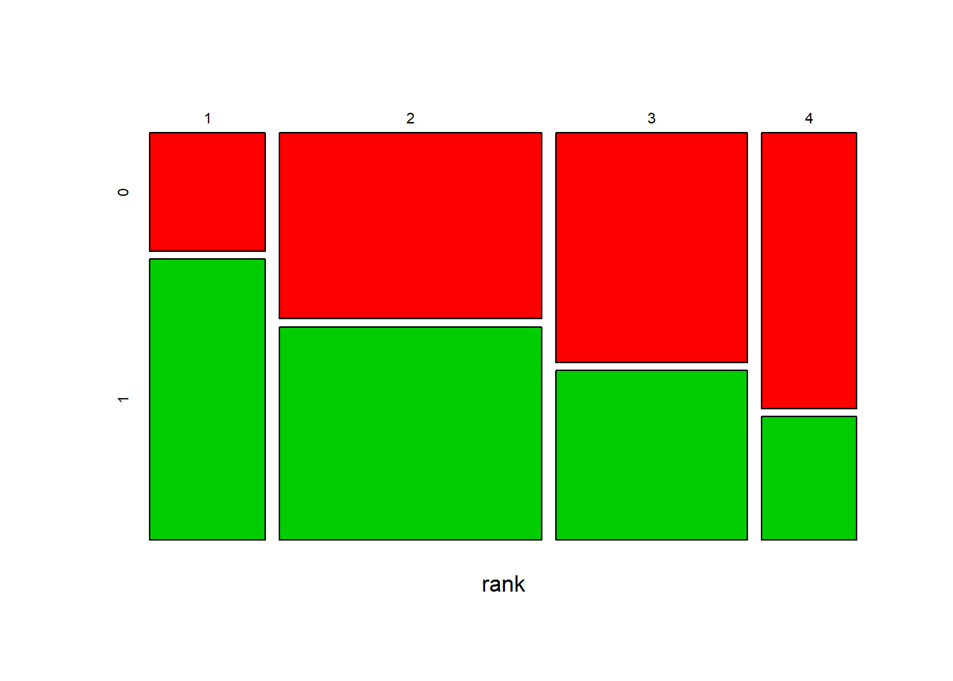
From the result above, we have A Priori probabilities to be admitted of 0.31: only 31% of the students were admitted to the program. Moreover, for numerical variables (gre, gpa) we have mean and standard deviation, and for categorical variables (rank) we have probabilities. For example, p(rank=1|admit=0)=0.103 and p(rank=1|admit=1)=0.245, as we can see from the result table above. We have also three plots of the model that represent the density for the numerical variables and the bars for the categorical variable.
# Prediction
p <- predict(model, data=train, type="prob")
head(cbind(p, train))
0 1 admit gre gpa rank
1 0.8449088 0.1550912 0 380 3.61 3
2 0.6214983 0.3785017 1 660 3.67 3
3 0.2082304 0.7917696 1 800 4.00 1
4 0.8501030 0.1498970 1 640 3.19 4
6 0.6917580 0.3082420 1 760 3.00 2
7 0.6720365 0.3279635 1 560 2.98 1# Confusion Matrix
p1 <- predict(model, data=train)
(tab1 <- table(p1, train$admit))
p1    0   1
  0 196  69
  1  27  33
# Missclassification
1 - sum(diag(tab1)) / sum(tab1)[1] 0.2953846From the table above, we can see that the first student has a probability of 0.84 to not be ammitted. If fact, admit=0, and he has low value of gre=380 and he came from a low rank=3. From the confusin matrix, we calculated a misclassification of 29%. In order to reduce the misclassification rate we can use the *Kernel. In fact, kernel based densities may perform better when numerical variables are not normally distributed.
# Naive Bayes Model
model <- naive_bayes(admit ~ ., data = train, usekernel = TRUE)
p2 <- predict(model, data=train)
tab2 <- table(p2, train$admit) # confusion matrix
1 - sum(diag(tab2)) / sum(tab2) # missclasification
[1] 0.2738462In fact, as we can see above, introducing the kernel based dentities the misclassification is reduced (from 29% to 27%).