Variable selection is an important aspect because it helps in building predictive models free from correlated variables, biases and unwanted noise. The Boruta Algorithm is a feature selection algorithm. As a matter of interest, Boruta algorithm derive its name from a demon in Slavic mythology who lived in pine forests.
How Boruta Algorithm works Firstly, it adds randomness to the given data set by creating shuffled copies of all features which are called Shadow Features. Then, it trains a random forest classifier on this extended data set (orignal attributes plus shadow attributes) and applies a feature importance measure such as Mean Decrease Accuracy, and evaluates the importance of each feature. At every iteration, Boruta Algorithm checks whether a real feature has a higher importance. The best of its shadow features and constantly removes features which are deemed highly unimportant. Finally, the Boruta Algorithm stops either when all features gets confirmed or rejected or it reaches a specified limit of random forest.
On the other hand, boruta find all features which are either strongly or weakly relevant to the response variable. This makes it well suited for biomedical applications where one might be interested to determine which human genes (predictors) are connected in some way to a particular medical condition (response variable).
library(Boruta)
library(mlbench)
library(caret)
library(randomForest)

data("Sonar")

# Feature Selection
set.seed(123)
boruta <- Boruta(Class ~ ., data = Sonar, doTrace = 2, maxRuns = 100) # number of interations
# print(boruta)
plot(boruta, las = 2, cex.axis = 0.7) # cex.axis is used to reduce the font size
plotImpHistory(boruta)
We use the Sonar datset that has 208 observations and 61 numeric variables apart from the Class variable which is a two level factor, where M stands for Mine (metal cylinder), and R stands for Rock.
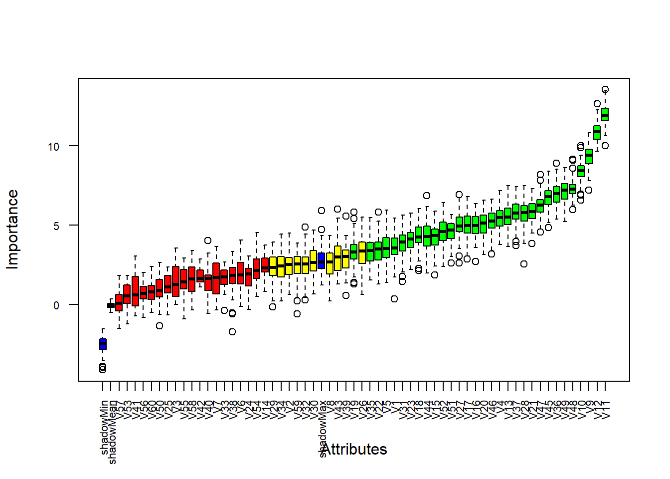
Ideally the importance of shadow attributes have to be close to zero, simply because the random fluctuation might has zero values. So, the shadow attributes could play the role of reference values for deciding which attributes are important. From the Box-Plot above the blue box-plot corrispond to the shadow attributes. We have three blue box-plot for the minimum, mean and maximum attribute. The green box-plots are confirmed important attributes, and red box-plots are confirmed to be unimportant. The yellow box-plots are tentatives, that means the algorithm was not able to arrive to a conclusion about their importance.
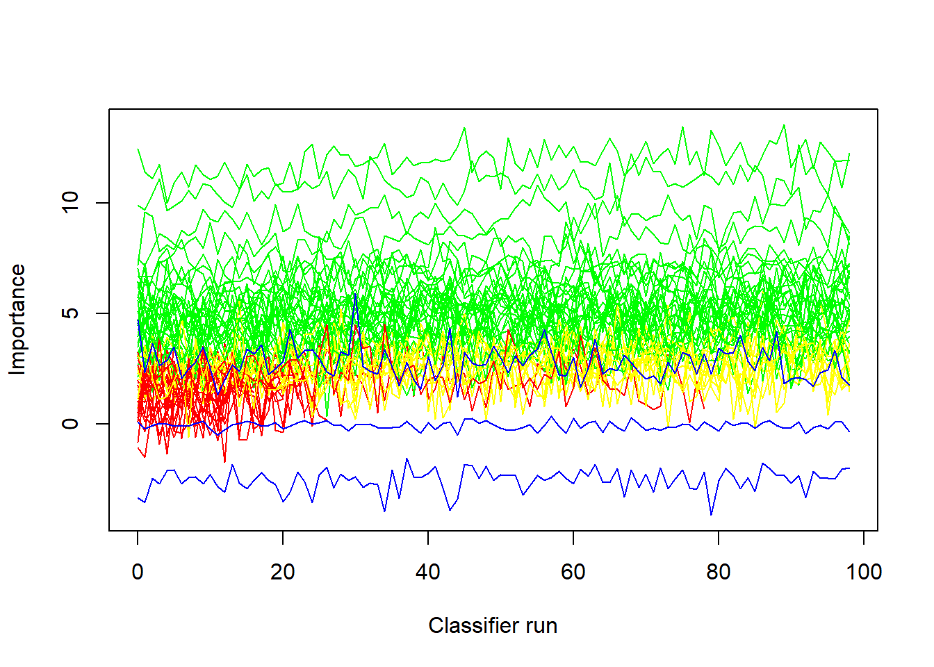
The last graph is the Importance History Graph, and we can see that the green attibutes have much higher importance than the shadow attributes depiced in blue. Now, we can try to find a soution for the Tentative attributes.
bor <- TentativeRoughFix(boruta)
print(bor)
Boruta performed 99 iterations in 29.47514 secs.
Tentatives roughfixed over the last 99 iterations.
32 attributes confirmed important: V1, V10, V11, V12, V13 and 27
more;
28 attributes confirmed unimportant: V14, V2, V24, V25, V29 and
23 more;# To have more information about the importance of attributes
# attStats(boruta)As we can see from the result above, 35 attributes are confirmed as important, and 25 attributes are confirmed as unimportant. Now, we can test if this feature selection with Boruta Algorithm has improved the performance of the random forest model.
# Data Partition
set.seed(123)
ind <- sample(2, nrow(Sonar), replace = T, prob = c(0.6, 0.4))
train <- Sonar[ind==1,]
test <- Sonar[ind==2,]

# Random Forest Model
set.seed(456)
rf60 <- randomForest(Class~., data = train)

# Prediction & Confusion Matrix - Test
p <- predict(rf60, test)
confusionMatrix(p, test$Class)
Confusion Matrix and Statistics
Reference
Prediction M R
M 35 13
R 6 27
Accuracy : 0.7654
95% CI : (0.6582, 0.8525)
No Information Rate : 0.5062
P-Value [Acc > NIR] : 1.513e-06
Kappa : 0.5298
Mcnemar's Test P-Value : 0.1687
Sensitivity : 0.8537
Specificity : 0.6750
Pos Pred Value : 0.7292
Neg Pred Value : 0.8182
Prevalence : 0.5062
Detection Rate : 0.4321
Detection Prevalence : 0.5926
Balanced Accuracy : 0.7643
'Positive' Class : M
Now the we have, from the code above, the random forest model with all the features included, we can compare it with the model that consider the feature selection made by the Boruta Algorithm. To do that we can use the function getNonRejectedFormula().
getNonRejectedFormula(boruta)Class ~ V1 + V2 + V4 + V5 + V8 + V9 + V10 + V11 + V12 + V13 +
V15 + V16 + V17 + V18 + V19 + V20 + V21 + V22 + V23 + V26 +
V27 + V28 + V29 + V30 + V31 + V32 + V34 + V35 + V36 + V37 +
V39 + V43 + V44 + V45 + V46 + V47 + V48 + V49 + V51 + V52 +
V59
<environment: 0x000000002971e850>set.seed(789)
rf41 <- randomForest(Class ~ V1 + V2 + V4 + V5 + V8 + V9 + V10 + V11 + V12 + V13 +
V15 + V16 + V17 + V18 + V19 + V20 + V21 + V22 + V23 + V26 +
V27 + V28 + V30 + V31 + V32 + V34 + V35 + V36 + V37 + V39 +
V43 + V44 + V45 + V46 + V47 + V48 + V49 + V51 + V52 + V59, data=train)
p <- predict(rf41, test)
confusionMatrix(p, test$Class)Confusion Matrix and Statistics
Reference
Prediction M R
M 35 11
R 6 29
Accuracy : 0.7901
95% CI : (0.6854, 0.8727)
No Information Rate : 0.5062
P-Value [Acc > NIR] : 1.277e-07
Kappa : 0.5795
Mcnemar's Test P-Value : 0.332
Sensitivity : 0.8537
Specificity : 0.7250
Pos Pred Value : 0.7609
Neg Pred Value : 0.8286
Prevalence : 0.5062
Detection Rate : 0.4321
Detection Prevalence : 0.5679
Balanced Accuracy : 0.7893
'Positive' Class : M
If we compare the result of the two models we can see that the original random forest has an Accuracy of 0.76, that is increase to 0.79 using the Boruta feature selection. So, we not only have a better model, but we also reduced the number of features.