Before the definition of the model it is always important to plot the distribution of our variable, finding unusual observation (points of leverage, hat value and outliers), missing data (understand if they are missing at random or not at random). Then, I always put the data in a multiple regression to see correlations and the presence of multicollinearity: is the phenomenon in which one predictor can be linearly predict from others with a substantial degree of accuracy. In this situation, the coefficients estimated may change erratically in response to small changes of the model. For this reason, I always test it using the Variance Inflation Factor Analysis VIF that test the ratio of variance in the model with multiple terms, dividing by the variance of the model with one term alone: so, it tests the severity of multicollinearity. Then, we can reduce the predictors finding the best ones using the Stepwise approach (comparing AIC and BIC index) and then the Relative Importance Weight Analysis: in multiple regression analysis, we are interested in determining the relative contribution of each predictor. The Relative Importance Weight Analysis, is a method by which we can partition the R-squared into pseudo-orthogonal portions. Each portion representing the relative contribution of one predictor variable.
Scale If we have to measure distances in KNN it is necessary to Scale the data. We can find opposite solution if we merely calculate distances without scaling. For example, we can use MixMax Scaler.
\[ X=(X-X \cdot \min ()) /(X \cdot \max ()-X \cdot \min ()) \] Another method is using the Z points, with mean=0 and standard deviation=1.
\[ X=(X-X . \text { mean }()) / X . s t d() \]
Outliers Linear models are influenced by Outliers. An observation is an outlier if it falls more than 1.5 IQR above the upper quantile or if it falls more than 1.5 IQR below the lower quantile. IQR is the Interquartile Range, is a measure of statistical dispersion, and is the difference between 75th and 25th percentiles: Q3-Q1.
Log-Transformation This move outliers closer to other values. For example, the log transformation drive outliers closer to the features’ average.
Feature Generation It is a process of creating. We can use One-Hot Encoding OHE to reshape the data in order to have 1 when the feature is present and 0 when is not present.
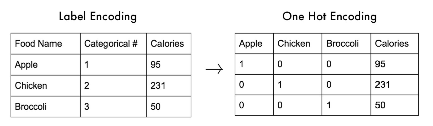
Crucially, One-Hot Encoding is by default already scaled. We can use the Sparse Matrix in order to exclude the 0s and work only when the feature is present, by doing that we save space in RAM. Note that we can use sparse matrix only if features with 0 are far less of all the values.
Anonymized Data Can happen that a company anonymize their data. Not only the values but also the column names could be anonymized: we can try to find relationship between columns or if they are grouped in some way. We can check the VIF to find multicollinearity.
Visual Exploration It is always the best way to look into data. Compare the overlapping of the kernel distributions between for example fraud vs. genuine credit card transactions. With Histograms we can also find how many values falls in to a bin. We can also observe if data are asymmetric, for example the distribution of money spent via credit card have by nature a right long tail.
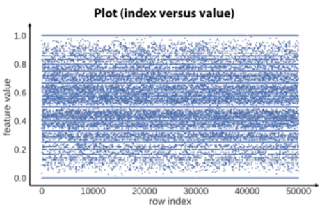
As we can see from the figure above, we can use Row Index vs. Feature Value to find Regularities in Missing Values or the frequencies over the values. We can also note the randomness over the indices. If fact, if we have horizontal patterns and not vertical patterns the data are randomly distributed.
IDD - Independent and Identically Distributed Which is to say all the data we have collected have not weirdness: test and train have the same distribution: that is a fundamental assumption.
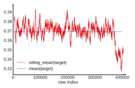
Shuffled Data By doing that, we can plot the values of a feature vs. row index and perform the rolling mean in order to smooth the values and better understand the trend. If the data are shuffled properly, we have to expect a sort of oscillation and no patterns are present around the average.
Missing Data Sometimes, missing data contain valuable information by themselves. In fact, we can have missing at random or missing data not at random. We can check it via shadow matrix. Shadow matrix is a method based on correlation. First, we replace the data in a dataset coding 1 for missing and 0 for present. Correlating these indicator variables with each other and with the original (observed) variables can help you to see which variables tend to be missing together.
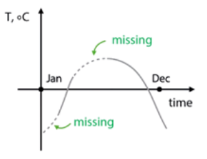
If we have data missing not at random, we can reconstruct missing values especially in time series by interpolation (the point that is on the curve derived from the actual data). We have also to consider that XGBoost can handle missing directly, also Mixed Models is robust to missing data.
Datetime and coordinates The datetime can be divided in time moment (e.g. day, month, year) in a period and time past from a particular event (time since, difference between dates). Time since a particular event: number of days left until last medication. Another example is when you have to estimate the risk of customer churn. Image he has last purchase date and the last call date, we can calculate the difference between them. About coordinate we can calculate the difference in distance between two important point in the Map. That is also crucial in Fraud Prevention, where we calculate how fast two purchases via credit card are made over a certain distance. Another measurable approach is to calculate the aggregated statistics, in this way, we can have an idea of high-price districts vs. low-price districts.
Validation & Cross Validation We need to split the data in train and validation part. There are many strategies in doing that. The questions is: how many splits? And which is the best method to perform such split? (holdout, leave-one-out, k-fold). The Leave-one-out Validation is a cross validation method. Let’s say we have 10 images, the performance of the model is tested on 9 of the 10 images. And so, we have a single-test-case that we can repeat 10 times, each time leaving out a different image. It is a very precise method, because each observation are used as test-set, but it requires quite a large computation time, in which case other approaches such as K-Fold Cross Validation may be more appropriate. The K-Fold Cross Validation can be viewed as a repeated holdout, because we split our data into K parts, using every part as validation set only once.
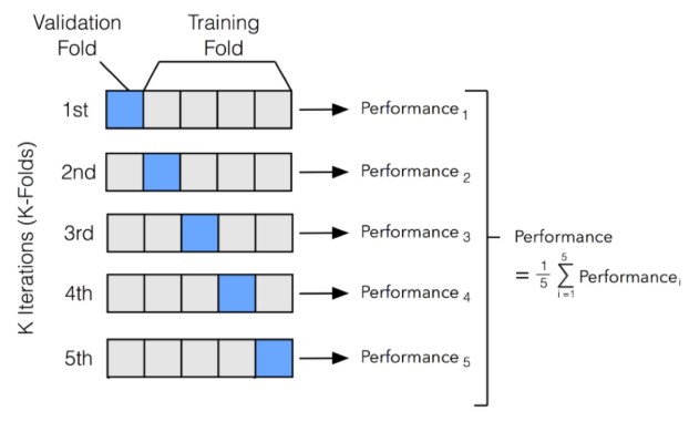
After this procedure, we average scores over these K-folds. The core idea is to use every sample for validate the results. To use this method is important to check if data are Shuffled.
If we have unbalanced data or multiclass classification (large amount of each class), Stratification is a way to insure we get similar target distribution over different folders. Stratification is a technique where we rearrange the data in a way that each fold has a good representation of the whole dataset. It forces each fold to have at least m instances of each class. This approach ensures that one class of data is not overrepresented especially when the target variable is unbalanced. For example in a binary classification problem where we want to predict if a passenger on Titanic survived or not. We have two classes here Passenger either survived or did not survive. We ensure that each fold has a percentage of passengers that survived and a percentage of passengers that did not survive.
If we have unbalanced data we can also use the Synthetic Minority Over-Sampling Technique SMOTE. In the presence of umbalanced dataset, we can have biased predictions and misleading accuracy. Like for example: 1 - credit cards frauds 2 - manufacturing defects 3 - rare diseases diagnosis We can solve this problem increasing the minority class or decreasing the majority class. We can keep the minority class as it is, and randomly remove majority class observations. The problem is that we could discard important information, and it may lead us to bias. Similarly in case of random oversampling, we randomly add more minority observations by copying some minority observations, for example, copying fraudulent transactions. But in this case, the mode is prone to overfitting due to copying same information.
In Time series cross-validation splitting time series data randomly does not help as the time-related data will be messed up. For time series cross-validation we use forward chaining also referred as rolling-origin. Origin at which the forecast is based rolls forward in time. In time series cross-validation each day is a test data and we consider the previous day’s data is the training set. From the figure below D1, D2, D3 etc. are each day’s data and days highlighted in blue are used for training and days highlighted in yellow are used for test.
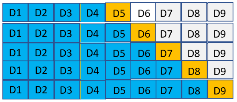
We start training the model with a minimum number of observations and use the next day’s data to test the model and we keep moving through the data set. This ensures that we consider the time series aspect of the data for prediction.