These are a series of analysis to illustate the main classification algorithms and their advantages.
The table shows the business clients of a company that has just launched a new product online. Some of the clients responded positively to the ads by buying the product and other responded negatively by not buying the product. The last column of the table tells for each user if the user bought the product or not.
| User.ID | Gender | Age | EstimatedSalary | Purchased |
|---|---|---|---|---|
| 15624510 | Male | 19 | 19000 | 0 |
| 15810944 | Male | 35 | 20000 | 0 |
| 15668575 | Female | 26 | 43000 | 0 |
| 15603246 | Female | 27 | 57000 | 0 |
| 15804002 | Male | 19 | 76000 | 0 |
| 15728773 | Male | 27 | 58000 | 0 |
| 15598044 | Female | 27 | 84000 | 0 |
| 15694829 | Female | 32 | 150000 | 1 |
Our mission is to use the main classifier algorithms and compare the best result. In this specific post we used Logistic Regression.
Splitting the dataset into the Training set and Test set.
library(caTools)
set.seed(123)
split = sample.split(dataset$Purchased, SplitRatio = 0.75)
training_set = subset(dataset, split == TRUE)
test_set = subset(dataset, split == FALSE)
Feature Scaling.
For classification is better to do feature scaling in order to have an accurate prediction.
Since most of the machine learning algorithms use Euclidian distance between two data point in their computations, this is a problem.
To supress this effect, we need to bring all feature to the same level of magnitudes. This can be achived by scaling.
dataset$Purchased = factor(dataset$Purchased, levels = c(0, 1))
training_set[-3] = scale(training_set[-3])
test_set[-3] = scale(test_set[-3])
Fitting Logistic Regression to the Training set.
classifier = glm(formula = Purchased ~ .,
                 family = binomial,
                 data = training_set)
Predicting the Test set results and Confusion Matrix at a cut-off of 0.5
prob_pred = predict(classifier, type = 'response', newdata = test_set[-3])
y_pred = ifelse(prob_pred > 0.5, 1, 0)

prob_pred = predict(classifier, type = 'response', newdata = test_set[-3])
y_pred = ifelse(prob_pred > 0.5, 1, 0)

cm = table(test_set[, 3], y_pred > 0.5)
Visualising the Test set results.
library(ElemStatLearn)
set = test_set
X1 = seq(min(set[, 1]) - 1, max(set[, 1]) + 1, by = 0.01)
X2 = seq(min(set[, 2]) - 1, max(set[, 2]) + 1, by = 0.01)
grid_set = expand.grid(X1, X2)
colnames(grid_set) = c('Age', 'EstimatedSalary')
prob_set = predict(classifier, type = 'response', newdata = grid_set)
y_grid = ifelse(prob_set > 0.5, 1, 0)
plot(set[, -3],
     main = 'Logistic Regression (Test set)',
     xlab = 'Age', ylab = 'Estimated Salary',
     xlim = range(X1), ylim = range(X2))
contour(X1, X2, matrix(as.numeric(y_grid), length(X1), length(X2)), add = TRUE)
points(grid_set, pch = '.', col = ifelse(y_grid == 1, 'springgreen3', 'tomato'))
points(set, pch = 21, bg = ifelse(set[, 3] == 1, 'green4', 'red3'))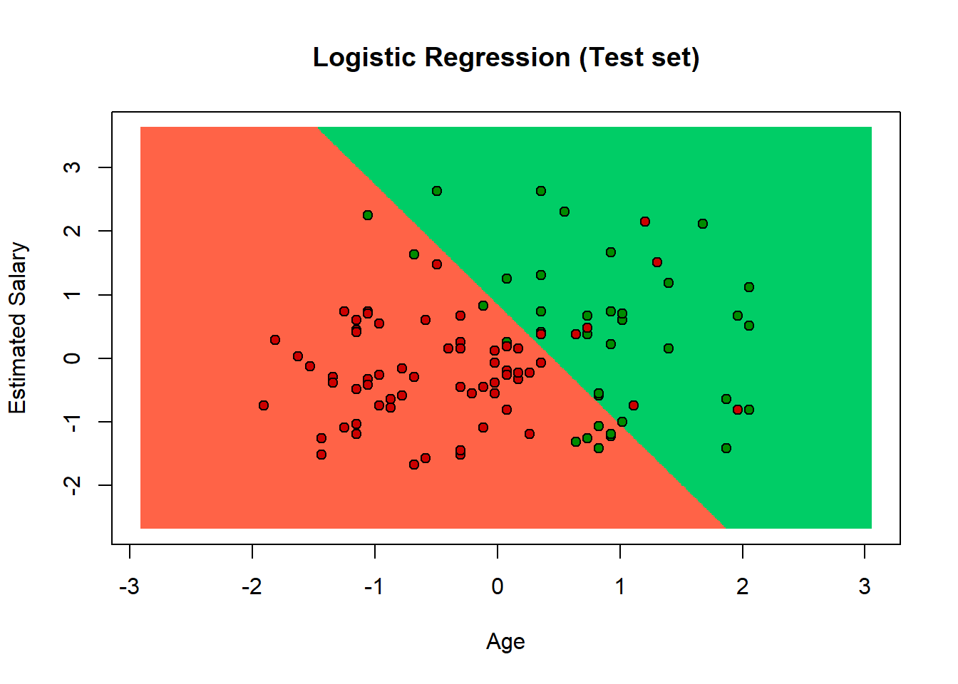
The prediction boundary is a straight line, in fact the logistic regression classifier is a linear classifier. So, the next graphs are related to a non-linear classifier and we will test if they have a better prediction.
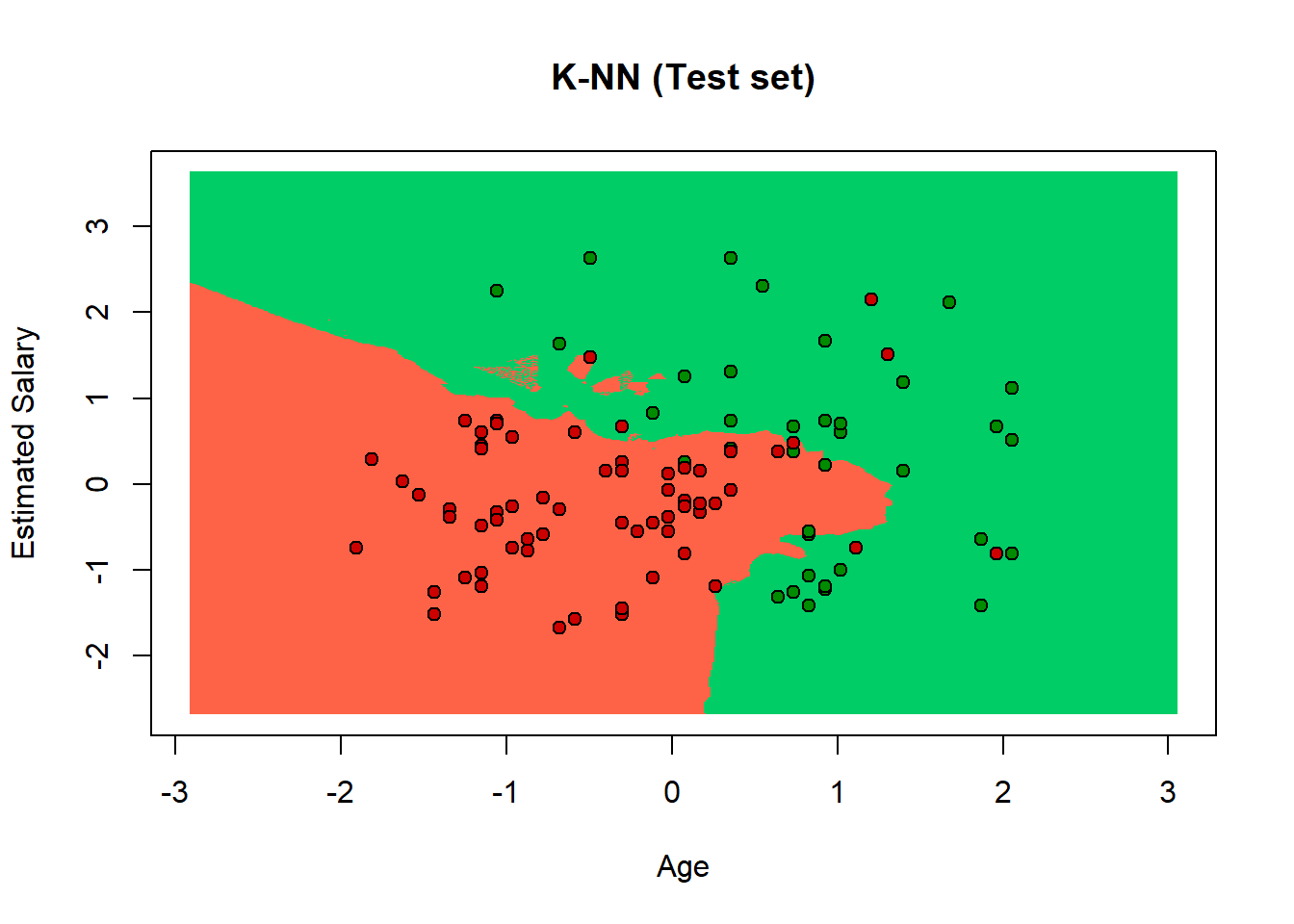
K-Nearest Neighbors K-NN It is an algorithm based on feature similarity. It is a non-linear classifier. It identifies the k nearest neighbors of a class that we want to estimate in its class. If we have k=3, the algorithm has to find the 3 nearest neighbors of the class. Choosing the right value of k is a process called parameter tuning, and is important to better accuracy. If the number of k is too low the bias is too small and we have a lot of noise. On the contrary, if the k is too big, then the process of estimation is too long. The solution is to use the square root of n where n is the total number of observations.
Kernel Suppor Vector Machine The goal of SVM is to design a hyperplane that classifies all the training vectors in two classes. We can have many possible hyperplanes that are able to classify correctly all the elements in the feature set, but the best choice will be the hyperplane that leaves the maximum margin from both classes. With margins we mean the distance between the hyperplane and the closest elements from the hyperplane. We use the Kernel trick when the categories are not linear separable. The Gaussian RBF Kernel is a function that represent a particular sigma function with the landmark in the middle of the space and is the point from where we measure the distance.

Random Forest Random Forests are built from Decision Tree. We can consider RM like a sort of Ensemble Learning. It is a non-linear and non-continuous regression model. How random forest works: 1 - Create a bootstrapped dataset with the same size of the original, and to do that Random Forest randomly selects rows with replacement. 2 - After creating a bootstrap dataset, we have to create a decision tree using he bootrapped dataset, but using only a subset of variables at each step.
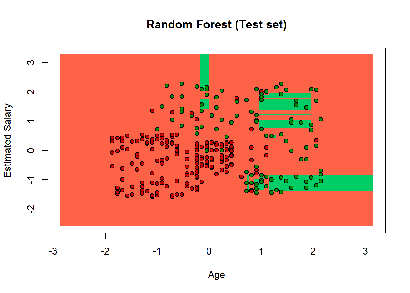
The Random Forest definitely catches most of the users that did not buy thenew launched product. But we have to be caresul because it is a bit overfitted. The problem of overfitting comes when we have too many features in the training set, even if the cost function can be close to zero, the model fails to generate the new sample.