Detect Scientific Topics using NLP

Studying related work within scientific literature is a crucial step in order to have a global overview about the scientific topics, but the amount of digital text data is growing exponentially and it is time consuming for researchers to find relevant information. Making scientific recommender systems smarter is crucial in order to help scientists in their bibliographical research phase.

How to tackle this problem to extract the topics: articles vs. abstract
The ambiguity is the most difficult problem in NLP. In fact, the same word can have different syntactic categories. For example in math the word “root” means square root, but in natural science it refers to the root of a plant. There is also a semantic problem because for example the word smoke could be related to a treatment for smoke cessation but also to an article on the relationship between smoking and the risk of cancer; here the subjects are in the same area (medicine) but they discuss different topics. So, we need to validate the context of the article and the context of the word, in order to provide the correct category. On the contrary, if two synonyms have two different concepts can cause redundancy.
It is also of high importance to define the term weight that characterize the article. If we got it wrong, the risk is to don’t represent the article accurately.
In order to minimize the problems described above, only the abstracts of the articles should be considered in the text analysis. The main reason is that the abstract is a brief but precise statement of the problem or issue, followed by a description of the major findings and conclusions reached. Moreover, it contains the most important key-words referring to the method and content: these should facilitate the topic analysis.

Data preprocessing of abstracts
In NLP a large part of the processing is Feature Engineering. In fact, we have to remove the noise to ensure efficient syntactic semantic text analysis for deriving meaningful insights from text. I discuss in much more detail the preprocessing step in python at this link.
Typically the steps are:

1 - Remove noise: such as numbers and punctuation using regular expressions.
2 - Regular Expression and Stemming: most of the cases the Snowball approach gives best results.
3 - Lemmatization: we need to have the inflected form of the word. For example the lemmatization of the word “ate” is “eat”.
4 - Minimum Edit Distance & Backtrace Method: is the way to correct grammar errors; maybe not necessary on scientific articles.
5 - Object Standardization: the acronyms are very present on scientific articles; we could decide if include them in the stop words list.
6 - Synonyms and antonyms: importing the Wordnet lexical database we can find words linked by their semantic relationship.
7 - Stop word removal: commonly used words in all articles such as “results”, “methods”, “conclusion” should be removed
8 - Bag of words & CountVectorizer: we count the number of occurrences for each word.

Bag of words is used to extract features and create the Term Document Matrix. To make the CountVectorizer more comparable, we scale it using the Term Frequency Transformation TF, and in order to boost the most important features we use the Inverse Document Frequency IDF, this calculate how often a word occurs in the corpus. The combination of both is called TFiDF = TF * IDF. This method reflects how relevant a term is in a given document.

Model Building
The most popular topic algorithm are:

1 - Latent Dirichlet Allocation LDA
2 - LDA2Vec

Problem to face in LDA & Parameter Tuning
The LDA is fat and easy to implement both in R and Python and gives much better results than a Vector Space Model VSM even when the cosine similarity in VSM is used. On the contrary, the limit of LDA is that it assumes a Gaussian distribution of the terms in the documents, which may not be true for all problems. Moreover, LDA involves Support Vector Decomposition, which is computationally intensive.
It is also of high importance to tune the parameters of LDA:

1 - Number of iterations.
2 - Number of Topics: number of topics to be extracted using Kullback Leibler Divergence Score.
3 - Number of Topic Terms: number of terms composed in a single topic.
4 - Alpha hyperparameter: represents document-topic density.
5 - Beta hyperparameter: represent topic-word density. The alpha & beta parameters are especially useful to find the right number of topics.
6 - Batch Wise LDA: another tip to improve the model is to use corpus divided into batches of fixed sizes. We perform LDA on these batches multiple times and we should obtain different results, but strikingly, the best topic terms are always present.

Data visualization to improve the model
Graph is always considered the first analysis. In this context the graphical representation is useful to check if the preprocessing steps are correct. Especially useful is the Co-Occurrence Matrix that indicates whether the two words co-occur or not.
Other tips to improve the results of LDA are:

1 - Frequency Filter: in order to get-rid of low frequency terms.
2 - Part of Speech Tag Filter: IN (prepositions), CD (cardinal numbers), MD (modal verbs) should be removed.

I discuss the theory of LDA in more detail at this link and a practical example in R at this link.

LDA vs. LDA2Vec
It is always a good idea to compare our initial model with one or more possible alternatives. A very promising approach is to use the LDA2Vec which is a hybrid algorithm combining best ideas from LDA and Word2Vec. At this link an explanation of Word2Vec.
The LDA2Vec is in every respect a deep learning of LDA. This approach combines global document themes with local word patterns The power of lda2vec lies in the fact that it not only learns word embeddings for words, but simultaneously learns topic representations and document representations as well:

1 - Word2Vec helps predict words inside a sentence: local prediction.
2 - LDA captures long-range themes beyond the scale instead of focusing over thousands of words: global prediction.

Crucially, LDA2Vec predicts globally and locally at the same time.

Conclusion
It is relatively simple to associate the abstract to the most probable topic, and then calculate the frequency per topic. In order to have a better estimate of the relative importance of each topic, the frequency should be weighted based on the impact factor of the journal were the article is published.
Other important aspects to take into consideration are:

1 - At the practical level, using LDA we can easily create human-readable topics.
2 - LDA2Vec in comparison of LDA requires much more computation and GPUs are needed.
3 - At the landing page of https://www.scilit.net/ there is the possibility to use the “search all fields” where a user can formulate a custom text as a search criteria which is a sort of “predict topic”. Crucially, if we want to rework our “topic models” with the predict topics over users then we might be interested in lda2vec.

Problem - 2b: Find closest author to a text using Science Network Analysis SNA
Having solved the Problem 1, we can use the Graph Theory methodology to create a “Science Network Analysis SNA” to analyze the relationship between Authors and Topics. We can also identify closets authors to a specific topic/text. Moreover, we can have a better understanding about how often an author writes an article and if he is an expert about one or more topics. The SNA approach has also the advantage to show the external collaboration between scientists using a graphical representation. A practical example using R and D3.js at this link.

The figure above is a simplify example of SNA filtered for the author a77. We have the following information:

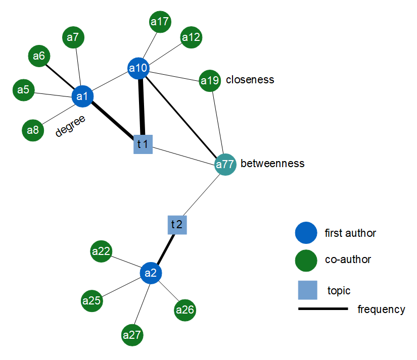
1 - co-authors (green node) and first authors (blue node) and their collaboration: represented by the link (black line).
2 - the relationship between topics (blue square) and their authors.
3 - external scientific collaborations (e.g. the link between a1 and a10).
4 - how often a scientist collaborate with other labs (e.g. the size of the link between a1 and a10).
5 - how many publications: represented by the size of the link (e.g. a10 has more publication than a1 on the same topic t1).

A case of serendipity
I would mention my personal scientific research represented by the a77 node. As we can see from the figure above, I worked as a co-author on neural activity on non-human primates t1 where the first author was the node a10. Moreover, I am first author about a treatment for smoking cessassions t2 (co-authors are not represented). Surprisingly, looking at my abstracts we can understand that there is a strong relationship between the bias of attention on monkey brain (t1: neural activity on non-human primates) and the bias of attention in smokers (t2: smoke treatment). This is a case of serendipity: the Science Network Analysis SNA was able to bring together two topics apparently distant from each other, helping the researchers to pursue the unexpected that is a stepping stone that lead to insights.

There are also many interesting metrics based on graph theory that can be calculated:

1 - betwenness centrality: the willingness to collaborate on different topics or with other labs.
2 - closeness centrality: how close is an author to emerging topics.

Many other centrality metrics exist, such as Eigenvector and PageRank. Each of these measures represents the importance of nodes, but we can also calculate “researcher communities” and their clusters’ identification.

Conclusion
There are many other solutions that can be used to find the influence of an author such as recommender system. The advantage in adopting Science Network Analysis SNA is that it gives a whole picture of the course of a web searching. Most importantly, we can play with the interactive SNA graph. See an example at the end of this article.