Multicollinearity is a phenomenon in which two or more predictors in a multiple regression are highly correlated (R-squared more than 0.7), this can inflate our regression coefficients. We can test multicollinearity with the Variance Inflation Factor VIF is the ratio of variance in a model with multiple terms, divided by the variance of a model with one term alone. VIF = 1/1-R-squared. A rule of thumb is that if VIF > 10 then multicollinearity is high (a cutoff of 5 is also commonly used). To reduce multicollinearity we can use regularization that means to keep all the features but reducing the magnitude of the coefficients of the model. This is a good solution when each predictor contributes to predict the dependent variable.
Ridge Regression performs a L2 regularization, i.e. adds penalty equivalent to square the magnitude of coefficients. Minimize the sum of square of coefficients to reduce the impact of correlated predictors. Keeps all predictors in a model. In Ridge Regression, we try to use a trend line that overfit the training data, and so, it has much higher variance then the OLS. The main idea of Ridge regression is to fit a new line that doesn’t fit the training data. In other words, we introduce a certain amount on bias into the new trend line. What we do in practice, is to introduce a Bias that we call LAMBDA, and the Penalty Function is: lambda*slope^2 The Lambda is a penalty terms and this value is called Ridge Regression or L2 and determines how severe the penalty. When LAMBDA = 0, the penalty is also 0, and so we are just minimizing the sum of the squared residuals. When LAMBDA asymptotically increase, we arrive to a slope close to 0. So, the larger LAMBDA is, our prediction became LESS sensitive to the independent variable. We use the BostonHousing dataset.
library(mlbench)
data(BostonHousing)
str(BostonHousing)
'data.frame': 506 obs. of 14 variables:
$ crim : num 0.00632 0.02731 0.02729 0.03237 0.06905 ...
$ zn : num 18 0 0 0 0 0 12.5 12.5 12.5 12.5 ...
$ indus : num 2.31 7.07 7.07 2.18 2.18 2.18 7.87 7.87 7.87 7.87 ...
$ chas : Factor w/ 2 levels "0","1": 1 1 1 1 1 1 1 1 1 1 ...
$ nox : num 0.538 0.469 0.469 0.458 0.458 0.458 0.524 0.524 0.524 0.524 ...
$ rm : num 6.58 6.42 7.18 7 7.15 ...
$ age : num 65.2 78.9 61.1 45.8 54.2 58.7 66.6 96.1 100 85.9 ...
$ dis : num 4.09 4.97 4.97 6.06 6.06 ...
$ rad : num 1 2 2 3 3 3 5 5 5 5 ...
$ tax : num 296 242 242 222 222 222 311 311 311 311 ...
$ ptratio: num 15.3 17.8 17.8 18.7 18.7 18.7 15.2 15.2 15.2 15.2 ...
$ b : num 397 397 393 395 397 ...
$ lstat : num 4.98 9.14 4.03 2.94 5.33 ...
$ medv : num 24 21.6 34.7 33.4 36.2 28.7 22.9 27.1 16.5 18.9 ...From the structure of the dataset shown above, we essentially have numerical data. We have a particular variable called mdev which is the median house price. As alredy said, Lambda=0 represents OLS and we have to find the optimum Lambda.
library(tidyverse)
library(broom)
library(glmnet)

# Define the responce variable
y = BostonHousing$medv
# Put all the predictors in a data matrix
x = BostonHousing %>% select(crim,zn,indus,chas,nox,rm,age,dis,rad,tax,ptratio,b,lstat) %>% data.matrix()

# Specify a range for Lambda
lambdas = 10^seq(3, -2, by = -.1)

# Ridge regression involves tuning a hyperparameter lambda, and it runs the model many times for different values of lambda
fit <- glmnet(x, y, alpha = 0, lambda = lambdas) # alpha=0 in ridge

# Use Cross Validation to find Best Lambda and how well the model generalises
cv_fit <- cv.glmnet(x, y, alpha = 0, lambda = lambdas)

# Lowest point in the curve indicates the optimal lambda
plot(cv_fit)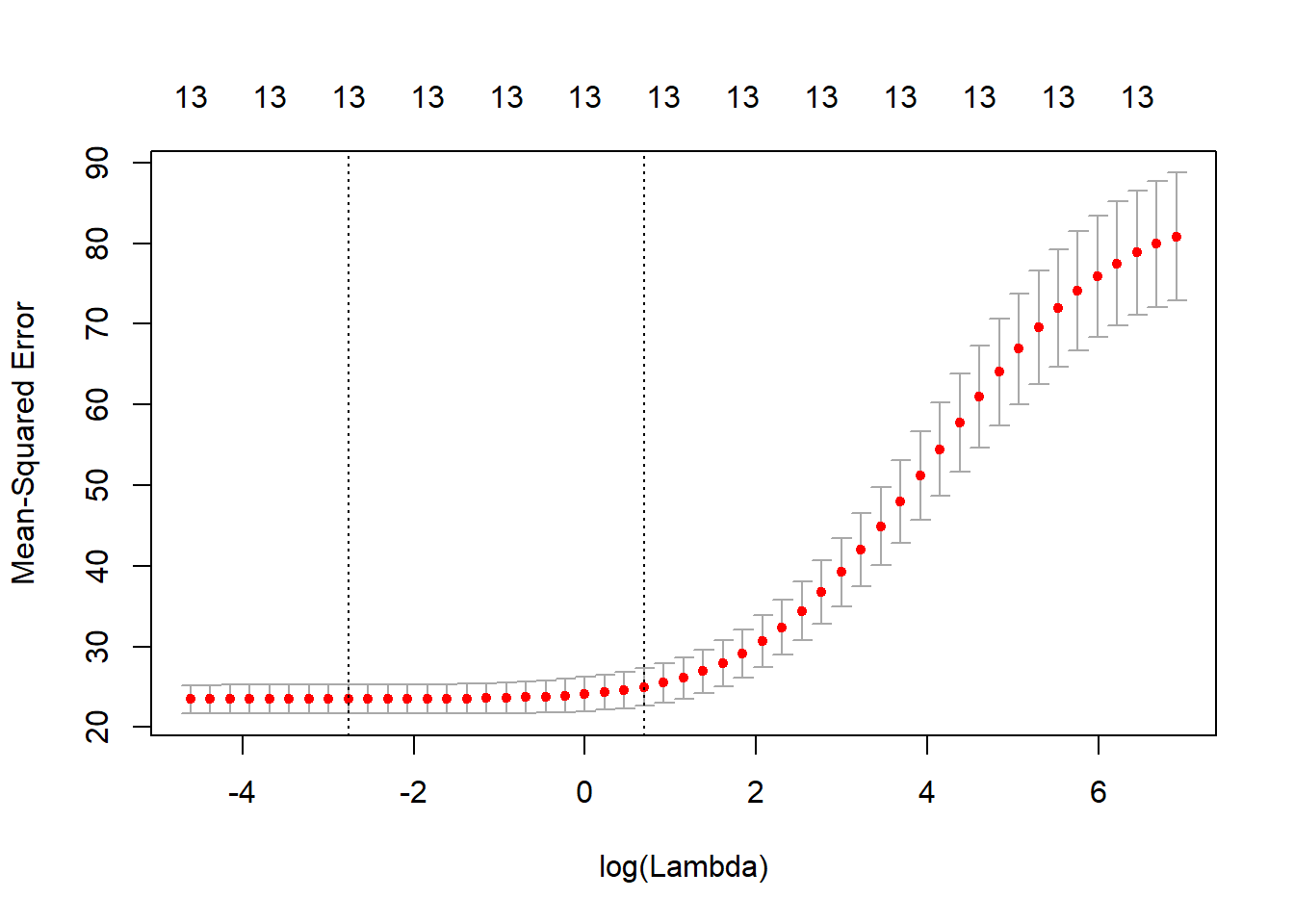
As we can see from the graph above, for low values of Lambda, the Mean Squared Error is quite low. On the contrary, as the value of Lambda increases, the Mean Squared Error also increases. So, we decide to continue using low value of Lambda.
optlambda <- cv_fit$lambda.min
optlambda # log value of lambda that best minimised the error
[1] 0.06309573The optimal value of Lambda to minimize the Error is 0.1 and we stored it in optlambda. So, we can now re-run the model using the optlambda value that we found.
# Predicting values and computing an R2 value for the data we trained on
 y_predicted <- predict(fit, s = optlambda, newx = x) # newx contanins the matrix of the predicted values

# Sum of Squares Total and Error
sst <- sum(y^2)
sse <- sum((y_predicted - y)^2)

# R squared
rsq <- 1 - sse / sst
rsq
[1] 0.9630046As we can see from the R-squared value rsq, now we have an optimal model that has accounted for 96% of the variance in the training set. We were able to obtain this result using all the predictiors, and we obtained a very good job in predicting house price, having a model that explain 96% of the variation n the house price.