Multicollinearity is a phenomenon in which two or more predictors in a multiple regression are highly correlated (R-squared more than 0.7), this can inflate our regression coefficients. We can test multicollinearity with the Variance Inflation Factor VIF is the ratio of variance in a model with multiple terms, divided by the variance of a model with one term alone. VIF = 1/1-R-squared. A rule of thumb is that if VIF > 10 then multicollinearity is high (a cutoff of 5 is also commonly used). To reduce multicollinearity we can use regularization that means to keep all the features but reducing the magnitude of the coefficients of the model. This is a good solution when each predictor contributes to predict the dependent variable.
LASSO Regression is similar to RIDGE REGRESSION except to a very important difference. The Penalty Function now is: lambda*|slope| The result is very similar to the result given by the Ridge Regression. Both can be used in logistic regression, regression with discrete values and regression with interaction. The big difference between Ridge and LASSO start to be clear when we increase the value on Lambda.
The advantage of this is clear when we have LOTS of PARAMETERS in the model: In Ridge, when we increase the value of LAMBDA, the most important parameters might shrink a little bit and the less important parameter stay at high value. In contrast, with LASSO when we increase the value of LAMBDA the most important parameters shrink a little bit and the less important parameters goes closed to ZERO. So, LASSO is able to exclude silly parameters from the model. We use the BostonHousing dataset.
library(mlbench)
data(BostonHousing)
str(BostonHousing)
'data.frame': 506 obs. of 14 variables:
$ crim : num 0.00632 0.02731 0.02729 0.03237 0.06905 ...
$ zn : num 18 0 0 0 0 0 12.5 12.5 12.5 12.5 ...
$ indus : num 2.31 7.07 7.07 2.18 2.18 2.18 7.87 7.87 7.87 7.87 ...
$ chas : Factor w/ 2 levels "0","1": 1 1 1 1 1 1 1 1 1 1 ...
$ nox : num 0.538 0.469 0.469 0.458 0.458 0.458 0.524 0.524 0.524 0.524 ...
$ rm : num 6.58 6.42 7.18 7 7.15 ...
$ age : num 65.2 78.9 61.1 45.8 54.2 58.7 66.6 96.1 100 85.9 ...
$ dis : num 4.09 4.97 4.97 6.06 6.06 ...
$ rad : num 1 2 2 3 3 3 5 5 5 5 ...
$ tax : num 296 242 242 222 222 222 311 311 311 311 ...
$ ptratio: num 15.3 17.8 17.8 18.7 18.7 18.7 15.2 15.2 15.2 15.2 ...
$ b : num 397 397 393 395 397 ...
$ lstat : num 4.98 9.14 4.03 2.94 5.33 ...
$ medv : num 24 21.6 34.7 33.4 36.2 28.7 22.9 27.1 16.5 18.9 ...From the structure of the dataset shown above, we essentially have numerical data. We have a particular variable called mdev which is the median house price. As alredy said, Lambda=0 represents OLS and we have to find the optimum Lambda.
library(tidyverse)
library(broom)
library(glmnet)

# Define the responce variable
y = BostonHousing$medv
# Put all the predictors in a data matrix
x = BostonHousing %>% select(crim,zn,indus,chas,nox,rm,age,dis,rad,tax,ptratio,b,lstat) %>% data.matrix()

# Specify a range for Lambda
lambdas = 10^seq(3, -2, by = -.1)

# LASSO regression involves tuning a hyperparameter lambda, and it runs the model many times for different values of lambda
fit <- glmnet(x, y, alpha = 1, lambda = lambdas) # alpha=1 in lasso

# cv.glmnet() uses cross-validation to work out
cv_fit <- cv.glmnet(x, y, alpha = 1, lambda = lambdas)
plot(cv_fit) # lowest point in the curve indicates the optimal lambda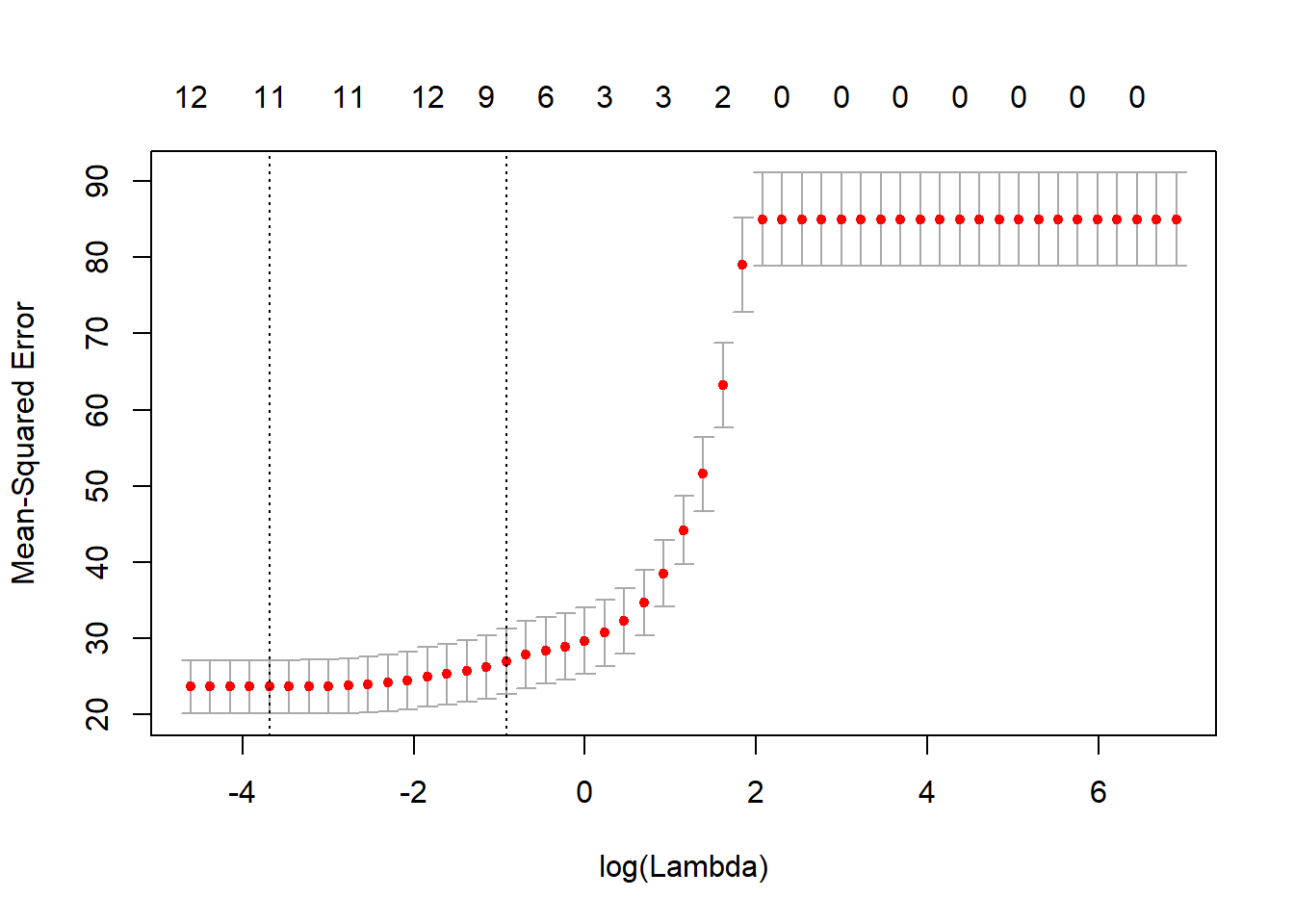
As we can see from the graph above, for low values of Lambda, the Mean Squared Error is quite low. On the contrary, as the value of Lambda increases, the Mean Squared Error also increases. So, we decide to continue using low value of Lambda.
optlambda <- cv_fit$lambda.min
optlambda # log value of lambda that best minimised the error
[1] 0.02511886The optimal value of Lambda to minimize the Error is 0.02 and we stored it in optlambda. So, we can now re-run the model using the optlambda value that we found.
# Predicting values and computing an R2 value for the data we trained on
 y_predicted <- predict(fit, s = optlambda, newx = x) # newx contanins the matrix of the predicted values

# Sum of Squares Total and Error
sst <- sum(y^2)
sse <- sum((y_predicted - y)^2)

# R squared
rsq <- 1 - sse / sst
rsq
[1] 0.9629666We found a n optimal model that has accounted for 96% of the variation of the responce variable in the training set. Pretty much like what we found in Rigre Regression. Both LASSO and Ridge Regression allow to use all the predictors to reach a robust regression model.