Customer segmentation via K-Means & Hierarchical clustering

Consider to have a big mall in a specific city that contains information of its clients that subcribed to a membership card. The last feature is Spending Score that is a score that the mall computed for each of their clients based on several criteria including for example their income and the number of times per week they show up in the mall and of course, the amount of dollars they spent in a year. the score goes from 0 (low spends) to 100 (high spends).

CustomerID	Genre	Age	Annual.Income..k..	Spending.Score..1.100.
1	Male	19	15	39
2	Male	21	15	81
3	Female	20	16	6
4	Female	23	16	77
5	Female	31	17	40
6	Female	22	17	76
7	Female	35	18	6
8	Female	23	18	94

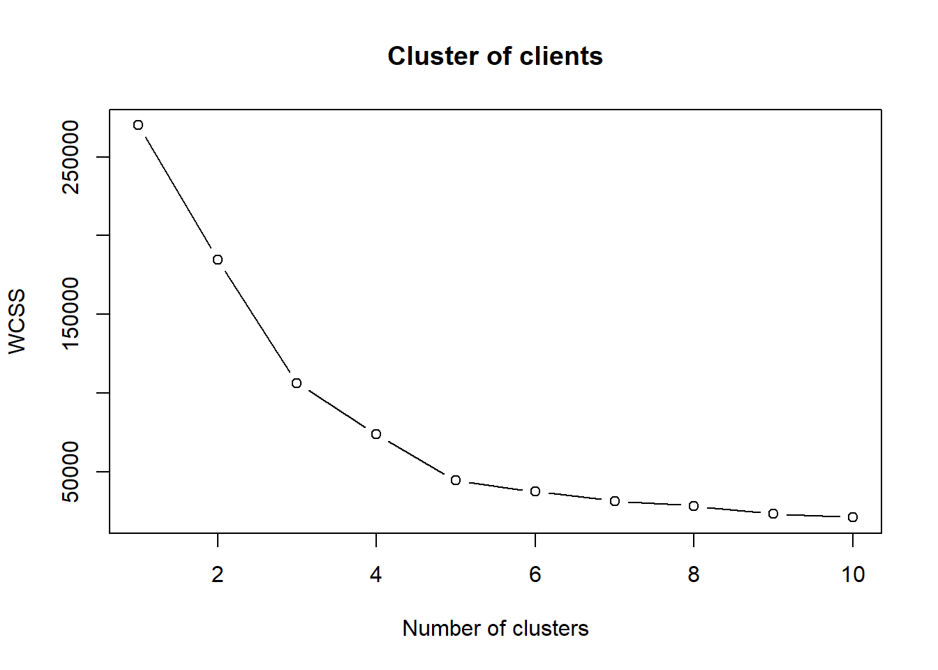
We have to segment the clients based on Annual Income and Spending Score. We sart using the K-Mean algorithm.
When we use K-Mean we have to specify the number of clusters. To do that, we use the Elbow Method to find the optimal number of clusters.

set.seed(6)
wcss <- vector()
for (i in 1:10) wcss[i] <- sum(kmeans(X, i)$withinss)
plot(1:10, wcss, type="b", main = paste('Cluster of clients'),
                           xlab = "Number of clusters",
                           ylab = "WCSS")

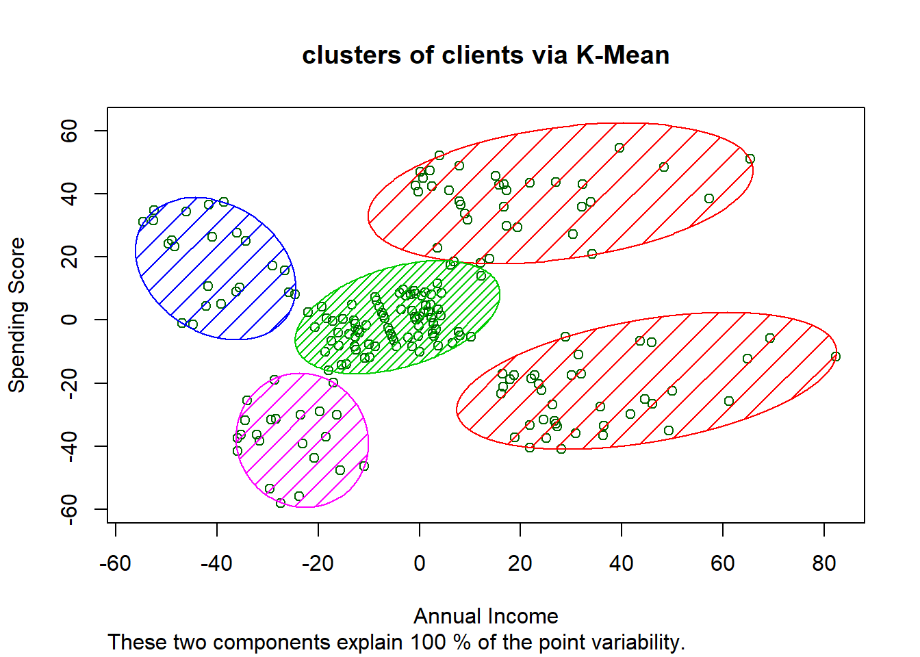
From the graph we see that the optimal number of clusters for our problem is 5 clusters. Now, we can apply K-Mean to the mall dataset.

set.seed(6)
kmeans <- kmeans(X, 5, iter.max = 300, nstart = 10)

library(cluster)
clusplot(X, kmeans$cluster,
            lines = 0,
            shade = TRUE, color = TRUE, labels = 0,
            plotchar = FALSE, span = TRUE,
            main = paste('clusters of clients via K-Mean'), xlab = "Annual Income", ylab = "Spending Score")

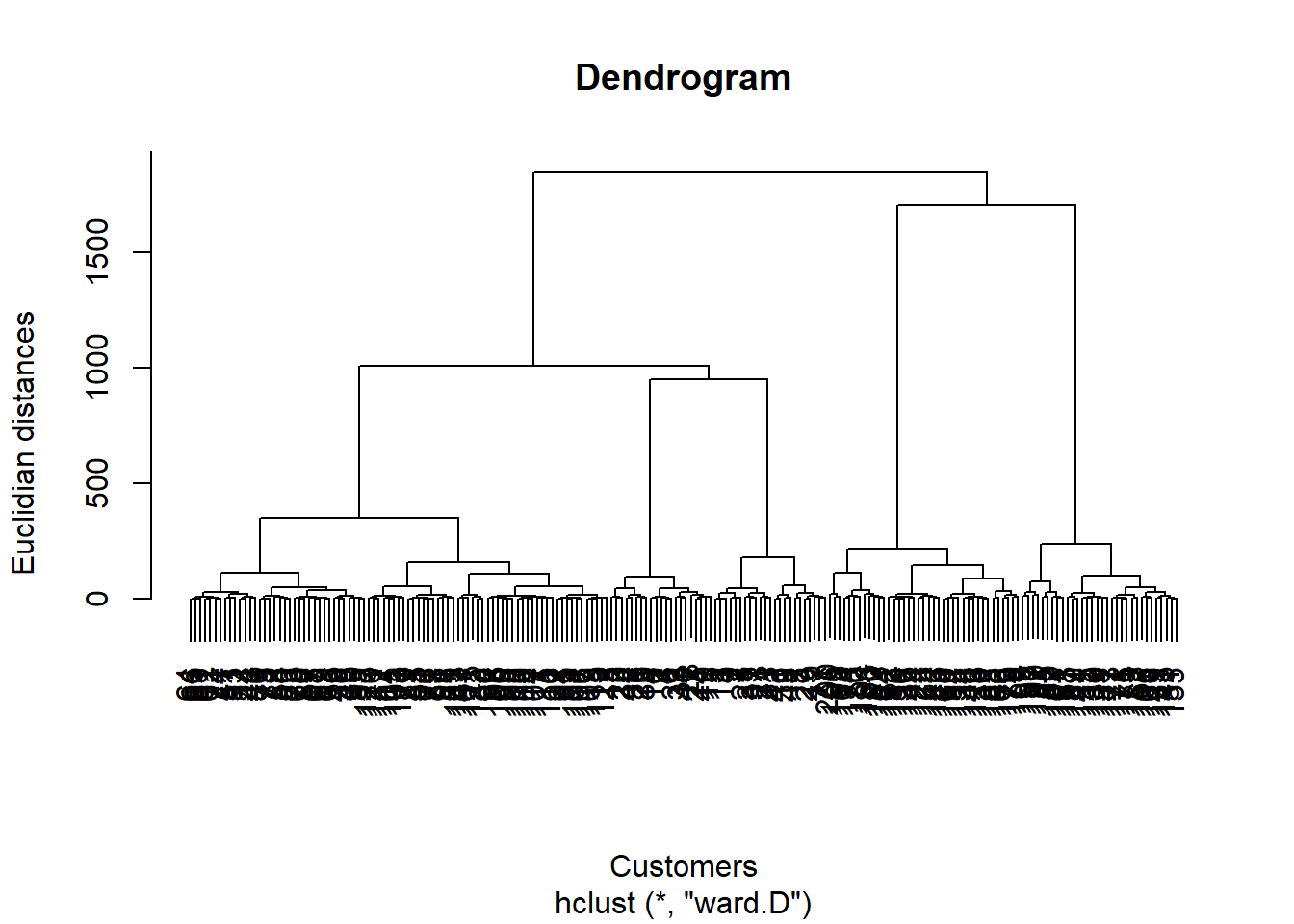
Now, more on performing Hierarchical Clustering. Firt, we use dendrogram to find the exact number of cluster, exactly like we did in the K-Mean.

dendrogram = hclust(dist(X, method = 'euclidian'), method = 'ward.D')
plot(dendrogram,
     main = paste('Dendrogram'),
     xlab = "Customers",
     ylab = "Euclidian distances")

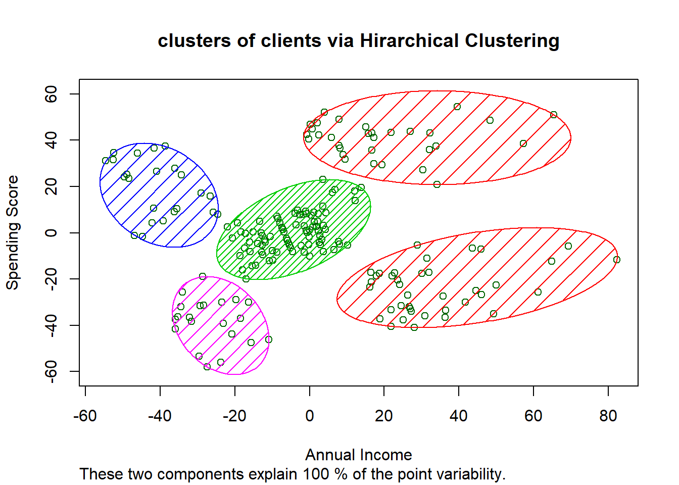
To find the optimal number of clusters, we need to find the largest vertical distance that we can make without crossing any other horizontal line. So, now we can fit our hierarchical clustering to the mall dataset. To do that here we use the Cut Tree method.

hc = hclust(dist(X, method = 'euclidian'), method = 'ward.D')
y_hc = cutree(hc, 5)

library(cluster)
clusplot(X, 
         y_hc,
         lines = 0,
         shade = TRUE, color = TRUE, labels = 0,
         plotchar = FALSE, span = TRUE,
         main = paste('clusters of clients via Hirarchical Clustering'), xlab = "Annual Income", ylab = "Spending Score")

The violet cluster has low income and low spending score. We can call them: SENSIBLE clients. The green cluster has both avrerage income and spending. We can call them: STANDART clients. The red top cluster has high income and high spending. They are the most targeting client in a compain: Target clients. The red bottom cluster has high income and low spending. We can call them: CAREFUL clients. The blue cluster has low income but high spending score. They do not care to spend much: CARELESS clients.