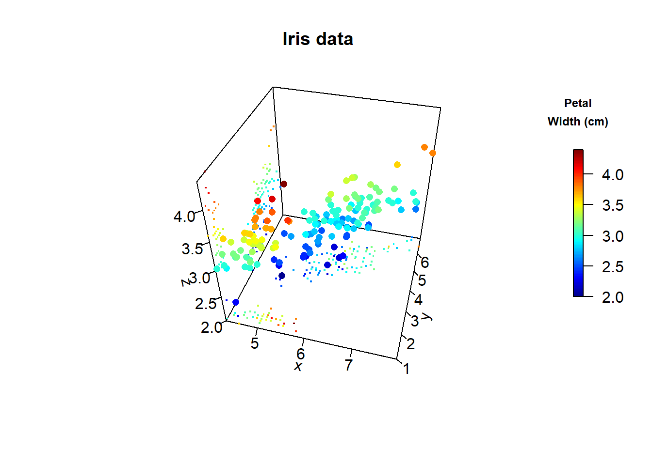
A 3D plot is quite popular, in particular in business presentation, but it is almost always inappropriately used. In fact, it is rare to see a 3D plot that could not be improved by turning into a regular 2D figure. Visualizations using 3D position scales can sometimes be appropriate, however. If the visualization is show it slowly rotation, rather than a static image from one prospective, will allow the viewer to discern where in 3D space different graphicla elements resides. The human brain is very good at reconstructing a 3D scene from a series of images taken from different angles, and the slow rotation of the graphic provides exactly these images. We’ll use the iris data set in the following examples.
# Load data
data(iris)
head(iris)
Sepal.Length Sepal.Width Petal.Length Petal.Width Species
1 5.1 3.5 1.4 0.2 setosa
2 4.9 3.0 1.4 0.2 setosa
3 4.7 3.2 1.3 0.2 setosa
4 4.6 3.1 1.5 0.2 setosa
5 5.0 3.6 1.4 0.2 setosa
6 5.4 3.9 1.7 0.4 setosa# Load libraries
library(plot3D)
library(rgl)
library(plot3Drgl)
# Define coordinates
x <- sep.l <- iris$Sepal.Length
y <- pet.l <- iris$Petal.Length
z <- sep.w <- iris$Sepal.Width
# Add small dots on basal plane and on the depth plane
scatter3D_fancy <- function(x, y, z,..., colvar = z)
{
panelfirst <- function(pmat) {
XY <- trans3D(x, y, z = rep(min(z), length(z)), pmat = pmat)
scatter2D(XY$x, XY$y, colvar = colvar, pch = ".",
cex = 2, add = TRUE, colkey = FALSE)
XY <- trans3D(x = rep(min(x), length(x)), y, z, pmat = pmat)
scatter2D(XY$x, XY$y, colvar = colvar, pch = ".",
cex = 2, add = TRUE, colkey = FALSE)
}
scatter3D(x, y, z, ..., colvar = colvar, panel.first=panelfirst,
colkey = list(length = 0.5, width = 0.5, cex.clab = 0.75))
}
# Define like color
scatter3D_fancy(x, y, z, pch = 16,
ticktype = "detailed", theta = 15, d = 2,
main = "Iris data", clab = c("Petal", "Width (cm)"))
In order to generate a fancy scatter plot with small dots on balsal palne the scater3D_fancu was created. We will create a simila function for histograms.
hist3D_fancy<- function(x, y, break.func = c("Sturges", "scott", "FD"), breaks = NULL,
                        colvar = NULL, col="white", clab=NULL, phi = 5, theta = 25, ...){

# Compute the number of classes for a histogram
  break.func <- break.func [1]
  if(is.null(breaks)){
    x.breaks <- switch(break.func,
                       Sturges = nclass.Sturges(x),
                       scott = nclass.scott(x),
                       FD = nclass.FD(x))
    y.breaks <- switch(break.func,
                       Sturges = nclass.Sturges(y),
                       scott = nclass.scott(y),
                       FD = nclass.FD(y))
  } else x.breaks <- y.breaks <- breaks

# Cut x and y variables in bins for counting
  x.bin <- seq(min(x), max(x), length.out = x.breaks)
  y.bin <- seq(min(y), max(y), length.out = y.breaks)
  xy <- table(cut(x, x.bin), cut(y, y.bin))
  z <- xy

  xmid <- 0.5*(x.bin[-1] + x.bin[-length(x.bin)])
  ymid <- 0.5*(y.bin[-1] + y.bin[-length(y.bin)])

  oldmar <- par("mar")
  par (mar = par("mar") + c(0, 0, 0, 2))
  hist3D(x = xmid, y = ymid, z = xy, ...,
    zlim = c(-max(z)/2, max(z)), zlab = "counts", bty= "g",
    phi = phi, theta = theta,
    shade = 0.2, col = col, border = "black",
    d = 1, ticktype = "detailed")

  scatter3D(x, y,
    z = rep(-max(z)/2, length.out = length(x)),
    colvar = colvar, col = gg.col(100),
    add = TRUE, pch = 18, clab = clab,
    colkey = list(length = 0.5, width = 0.5,
       dist = 0.05, cex.axis = 0.8, cex.clab = 0.8)
       )
  par(mar = oldmar)
}


# Create his3D using plot3D
# hist3D_fancy(iris$Sepal.Length, iris$Petal.Width, colvar=as.numeric(iris$Species))

# Make the rgl version
# plotrgl()
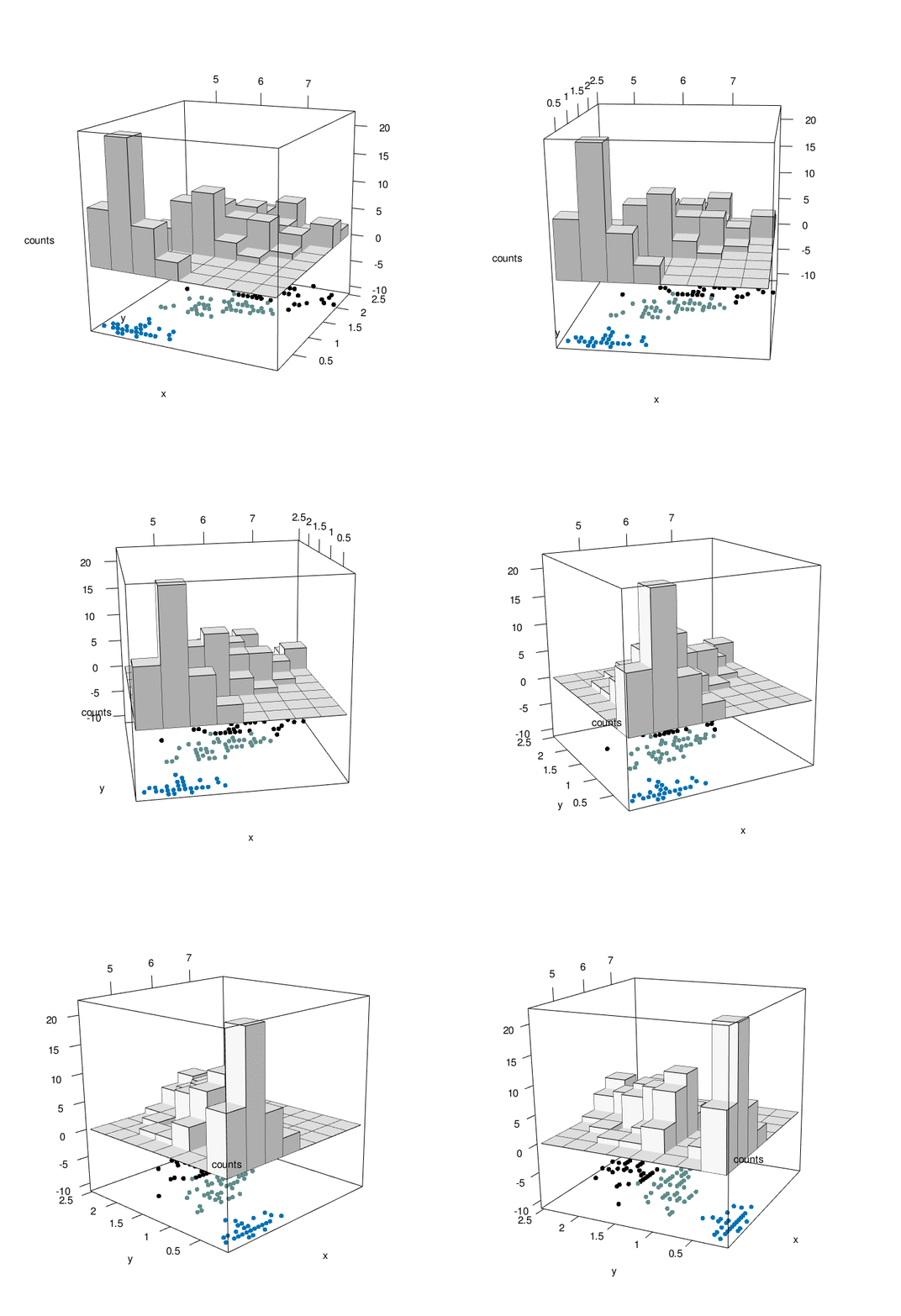
Looking at the graph above, we can have a comprehensive view of 4 characteristic of iris flowers in the same graph. At the bottom, We have the relationship between iris sepal lenght and iris petal width as a function of the three differenc species (setosa=1, versicolor=2, virginica=3). At the top of the graph, we can appreciate the counting of iris sepal lenght crossed with iris petal width (divided in bins). The slow animation helps to better understand all the dynamics involved.