The tuning process is a painful process in deep learning because we have many paramters: 1 - alpha learning rate 2 - the momentum beta 3 - beta1, beta2, epsilon in AdaM 4 - number of layers L 5 - number of hidden units 6 - learning rate decay parameters 7 - mini-batch size
Some of these paramters reported above, are more impotant than others. The learning rate alpha is the most important parameter to tune.
First just remind what is the learning rate: Stochastic gradient descent is an optimization algorithm that estimates the error gradient for the current state of the model using examples from the training dataset, then updates the weights of the model using the back-propagation of errors algorithm, referred to as simply backpropagation. The amount that the weights are updated during training is referred to as the step size or the learning rate. Specifically, the learning rate is a configurable hyperparameter used in the training of neural networks that has a small positive value, often in the range between 0.0 and 1 .
The second important parameters are beta for momentum, mini-batch size and the number of hidden units. The thrid most important are learning rate decay and the number of layers.
It is a common pratice to sample the parameters at random using grid search, and systematically explore the values. This is good in machine learning, but when we have to deal with high number of hyperparameters it is recommended to choose the points in grid search at random. In fact, it is overly complex to know in advance which hyperparameters ae going to be the most important for our problem.
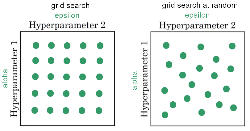
From the figure above we are trying to tune just two parameters: alpha and epsilon. It is quite evident the advantage to use the random grid search. In fact, using grid searchwe are using five values of alpha and all the different values of epsilon give back the same answer; we trained 25 models and only 5 values of epsilon. In contrast, the random grid search give back 25 learning rate of both alpha and epsilon. We have to consider also that in reality, we have to tune more than two hyperparameters, and using grid search at random give a more richy exploring set of possible values.
Coarse to fine method We can find that there are specific points that work the best and we can zoom-in to this smaller area of values as depicted in the figure below.
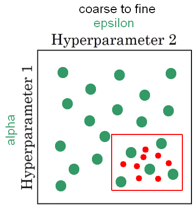
After we defined the new square region, we can try to use more values (colored in red). Now, we have amore density with in the most promising area of bes values to use in our model. that are again at random, but we are focused more resources on searching within a area that is suspecting that the best setting of parameters is in this region.
How to choose the appropiate scale Sampling using grid search at random, over the range of hyperparameters, can allow us to search over the space of hyperparameters more efficiently. On the contrary, sampling at random doesn’t mean sampling uniformly at random over the range of valid values. Instead, it is important to pick the appropriate scale on which to explore the hyperparameters. For example, if we have to choose the number of layers, we can consider a range from 2 to 6 and in this case grid reach could be a reasonable method. Anothe example is when we are seareching for the approproate learning rate alpha that goes from 0.0001 to 1. A sample value uniformly at random over this range could be to use the 90% of the resorces between 0.1 to 1 and 10% of resources between 0.0001 to 0.1. A good alternative is to use the linear scale where we use random sample from 0.0001 to 0.001 and again random from 0.001 to 0.01, and from 0.01 to 0.1, and again random from 01. to 1. Using the linear scale method we have more resources dedicated between fixed ranges.
Batch Normalization When we train a model, normalizioing the input features can speed up the learning process. In a deep neural neetwoek we have to train mant hidden layers; normalizing the values of the preavious hidden layer make the training of next hidden layer easier. It is common to normalize after the activation function a and before the activation function z, but z happen more often. Given some intermediate values in the neural network from z^1 to z^n, we can perform the following calculation:
\[ \begin{array}{l}{\mu=\frac{1}{n} \sum_{i} z^{(i)}} \\ {\sigma^{2}=\frac{1}{n} \sum_{i}\left(z_{i}-\mu\right)^{2}} \\ {z_{n o r m}^{(i)}=\frac{z^{(i)}-\mu}{\sqrt{\sigma^{2}+\varepsilon}}} \\ {\hat{z}^{(i)}=\gamma z_{\text {norm}}^{(i)}+\beta}\end{array} \] From the calculation above, we compute the normalization for the mean and variance, and than we used that values to normalize the values of the hidden layer before the activation function called z. By doing this we have z with mean 0 and variance equal to 1. If we don’t want to have every hidden units with mean 0 and variance 1, we can make gamma + beta (see last formula above). Here, gamma and beta are learnable parameters. After this normalization we can fit the activation function in order to get a. The Batch Normalization is used in combination of Mini-Batch of our training-set.
Reference: coursera deep neural network course